Example VTune Analysis

As an example we use VTune Amplifier to analyze the performance of the original, and the optimized software package ART - a 3D radiative transfer solver developed within the SolarALMA project. The code is written in C++ and consists of two major computational parts:

• An equation of state (EOS) solver, which - based on various types of input data - computes electron density, gas pressure, and density.

• A nonlinear solver for radiative transfer (RT). This code is based on a FORTRAN code from 1970 by Robert Kurucz.

Input data is read from HDF5 files and composed into a set of 3D Cartesian grids. The two kernels described above are executed independently for each grid point, with no communication required by the neighbor cells. In this sense the code is trivially parallelizable and to find opportunities for optimization we look at the per-core (call it “sequential”) performance. The optimization effort has been done within the PRACE Preparatory Access project type D. For more details about the optimizatoin techniques consult the white paper.

Using VTune on Fram

First, to use VTune on Fram you need to load the corresponding software module VTune. To list the available versions:

$ ml avail VTune

   VTune/2017_update1    VTune/2018_update1    VTune/2018_update3

Then load the desired (newest) version

$ ml load VTune/2018_update3

To gather information about a code’s performance one needs to execute the code using the amplxe-cl command. Depending on the needs, amplxe-cl can gather all sorts of performance statistics: FPU utilization, usage of vector (SIMD) AVX insturctions, instructions per clock, memory bandwidth, cache utilization, threading level, etc. For example, to collect general information about the most time-consuming parts of the code:

$ amplxe-cl -collect hotspots ./your-program your-arguments

For a complete list of analysis modes please consult the VTune documentation. A useful set of performance metrics is gathered by the hрc-performance analysis, which can help to identify opportunities to optimize CPU, memory, and vectorization level:

$ amplxe-cl -collect hpc-performance ./your-program your-arguments

A detailed description and the available options for each profiling mode can be obtained as follows

$ amplxe-cl -help collect hpc-performance

[...]

 To modify the analysis type, use the configuration options (knobs) as
 follows:
 -collect hpc-performance -knob <knobName>=<knobValue>
 Multiple -knob options are allowed and can be followed by additional collect
 action options, as well as global options, if needed.

sampling-interval
[...]

enable-stack-collection
[...]

collect-memory-bandwidth
[...]

dram-bandwidth-limits
[...]

analyze-openmp
[...]

The enable-stack-collection knob, disabled by default, provides detailed caller / callee information for each profiled function. It can be very useful, but might introduce some overhead. We will use it in the following example.

Collected performance statistics are saved in a subdirectory, by default in the directory you are running from. For the above example the results are stored in r000hpc/. They can then be compressed and moved to, e.g., a desktop computer, or they can be analyzed on one of the Fram login nodes using the VTune Amplifier GUI:

$ ssh -Y fram.sigma2.no
$ ml load VTune/2018_update3
$ amplxe-gui

Note that running the GUI directly on Fram migh feel sluggish depending on your network connection.

VTune analysis

The performance characteristics of the original code are obtained as follows

amplxe-cl -collect hpc-performance -knob enable-stack-collection=true -knob collect-memory-bandwidth=false mpirun -np 1 ./ART.x

Since we are interested in the “sequential” (per-core) performance, we only analyze a single MPI rank. The stack collection is enabled. Once the sampling results are opened in the VTune Amplifier GUI, the performance summary is presented:

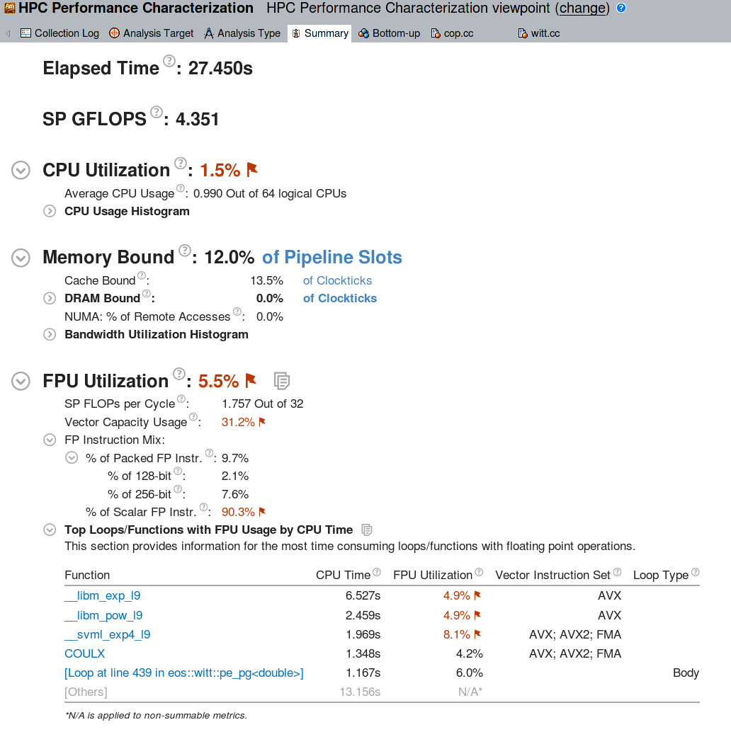
The CPU Utilization section shows the total percentage of all available cores used. Since a single ART process was executed, this metric is very low (1 out of 64 logical cores are used), but that is expected. The memory statistics show that ART is compute bound: there is almost no references to the global memory (DRAM bound 0%). Also the caches are not very busy. It is clear that most of the run time goes into CPU instructions.

The FPU utilization report is hence the most interesting one in this case. It reveals that 90% of the floating point instructions are scalar, i.e., the vector units (AVX) are mostly unused. Looking at the top most busy functions it becomes clear that the time is spent in calls to libm exp and log.

A closer look at the Bottom-up section of the performance report reveals the heaviest parts of the code.

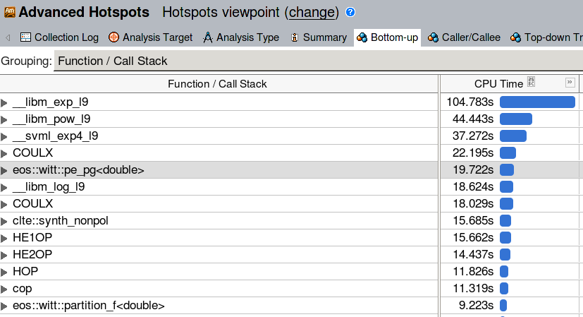
This confirms the previous finding (and adds pow to the list of computationally heavy functions). From the above reports we can roughly sketch the optimization directions:

• Re-write the code such that the vectorized math library is used for exp, log, pow calls

• Concentrate on the heaviest functions from the Bottom-up list

The optimized code

Both GCC and ICC provide an interface to a vectorized math library with platform-optimized implementations of amongst others exp,pow,log. Intel compiler uses its own Short Vector Math Library (SVML). The library comes together with the compiler installation, and there is nothing system-specific that needs to be done to use it. GCC on the other hand relies on libmvec, which is part of Glibc version 2.22 and higher. This means that on systems with an older version of Glibc the vectorized math library is not readily available, regardless of the GCC version. This is a practical problem, because OS vendors often lag a few years when it comes to Glibc (e.g., Centos 7.5 comes with version 2.17 released in the end of 2012). However, it is possible to install a custom Glibc as a module and use it for user’s code.

As noted in the documentation of SVML the vectorized math library differs from the scalar functions in accuracy. Scalar implementations are not the same as the vectorized ones with vector width of 1. Instead, they follow strict floating-point arithmetic and are more computationally demanding. GCC is by default conservative wrt. the floating-point optimizations: vectorized math library is only enabled with the -ffast-math compiletime option. ICC by default uses relaxed settings (-fp-model fast=1), which allow the compiler to make calls to low accuracy SVML functions. In addition, SVML also provides higher accuracy vectorized functions (-fp-model precise). Vectorization of libm calls can be prohibited with -fp-model strict. With ART the high accuracy is not required, hence we compile the code with the most relaxed settings.

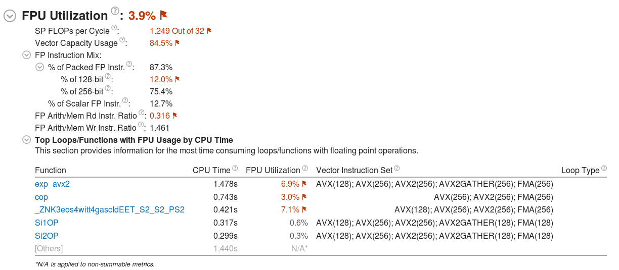
Vectorization of the code has been performed using #pragma simd defined by the OpenMP standard. All the heaviest ART functions, and all floating-point intensive loops have been vectorized using this method, and VTune was used throughout the process to find new bottlenecks once the existing ones have been optimized. Below is the final VTune report of the optimized code compiled using the GCC 8 compiler:

and using the Intel 18 compiler:

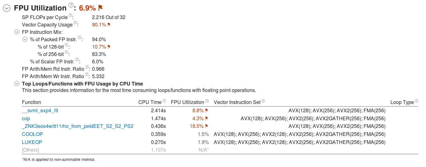
Notably, the optimized code utilizes the vector (AVX) units for 87% of the total FP instructions with GCC, and for 94% of the FP instructions with the Intel compiler. The capacity of the vector units is used in 85%-90%, which demonstrates that the code is almost fully vectorized.

Compared to the original code, the performance tests have shown that on a Broadwell-based architecture the optimized code works from 2.5 times faster (RT solver) to 13 times faster (EOS solver) on a single core. All optimizatoin techniques employed have been described in detail in the white paper.