Tuning applications

Introduction

Running scientific application in order to maximise the efficiency of the hardware is increasingly important as the core count increase. A system like Betzy with 172k cores represent a substantial cost and efficiency of the applications run should be as high a practically possible.

There are several steps with increasing complexity that can be taken to learn more about the application’s behaviour. Starting from checking the scaling to produce a roof line model of the application. Digging deeper into the matter is also possible with even more advanced usage of the tools and even more advanced tools.

A set of tools is presented, each with increasing complexity.

In this case study we’ll follow a real application called FVCOM which is an ocean current simulation code. I typically run on 1024 cores, not the application with the highest core count, but a typical example of a seasoned well known application with it’s special traits.

In the following we will cover application tuning and benchmarking at a general level. If you are interested in specific advice or guidance for your particular software, please have a look at the application specific pages, locate your application and see if it has a dedicated guide. If not, and this is of interest to you, please consider contacting us by sending a mail to support@nris. We greatly appreciate any assistance or help in improving this.

Scaling

The scaling of an application is one of the key factors for running in parallel. This simple metric is very simple to record. Just run the application with an increasing number of cores and record the run time (many ways exist to record run time, but time -p mpirun <executable> is one of the simplest. As the speedup in many cases also depend on the input data used it is important to run the scaling test with a relevant input data set.

Plot the recorded run time as function of core used and look for trend in the run time, alternatively plot the speedup from the lowest core count.

# cores	run time	speedup
128	4071.89	1
256	2193.52	1.86
512	1173.19	3.47
1024	659.38	6.18
2048	395.53	10.29

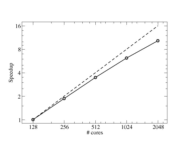
Fig. 1 - Scaling

The plot show the recorded speedup for FVCOM with the current input data. The dashed line represent perfect speedup.

ARM Performance reports

To learn a great deal of the application the tool Performance-reports can be used. This tool profile the application and provide a one page report with a huge array of important metrics.

Running

The commands used to run the ARM performance reports are:

module load Arm-PerfReports/20.0.3
perf-report mpirun ./fvcom.bin --casename=$RUN > $RUN_DIR/log-${SLURM_JOBID}.out

When the Slurm job is finished two files containing performance reports are found as: fvcom_1024p_8n_1t_yyyy-mm-dd_hh-mm.txt and fvcom_1024p_8n_1t_yyyy-mm-dd_hh-mm.html.

See also How to check the performance and scaling using Arm Performance Reports.

Header

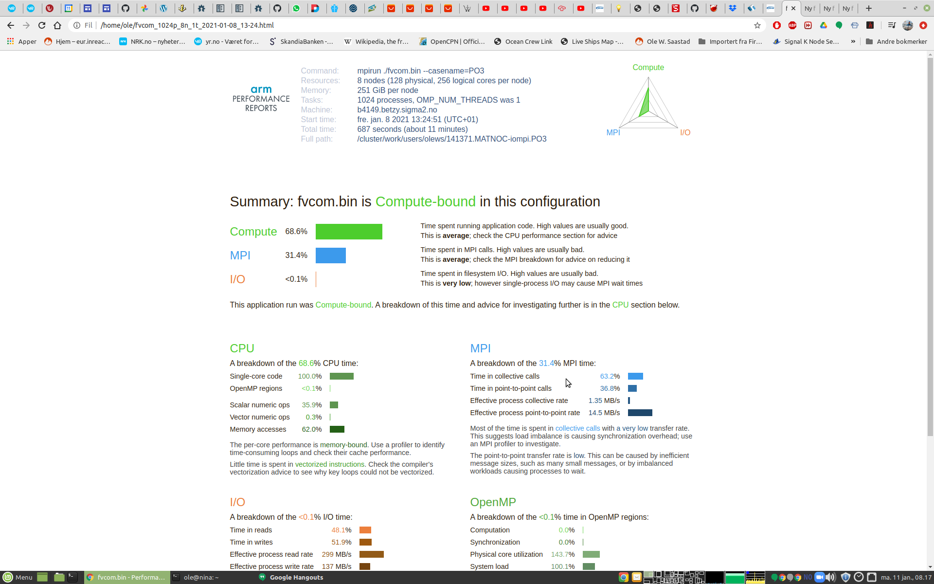
Fig. 2 - Performance report header

The header give basic information how the application was invoked and run. It also provide total wall time. The figure to the right give a quick overview of how the time is distributed over the categories of execution. This is binned into 3 categories, compute time, time spent in MPI library and time spent doing Input & Output. In this example we see that time is spent on doing computation and communication using MPI.

Summary

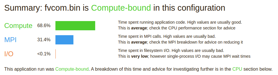
Fig. 3 - Performance report summary

The summary report section contain a lot of useful information in just a few lines. It show us that only 69% of the time is spent doing computations. This metric is important when we calculate the total efficiency of the application.

The next entry teach us that the application spent 31% of the total time doing communication using MPI. This is time spent as a consequence of MPI functions needed to make a parallel program. This number should be as low as possible as the time spend doing communications is wasted compute cycles. About 1/3 of all compute cycles in this run is wasted do to waiting for MPI functions t complete.

The last entry show that FVCOM does very little Input & Output during a run. Other applications might have a far larger number here.

Details - CPU

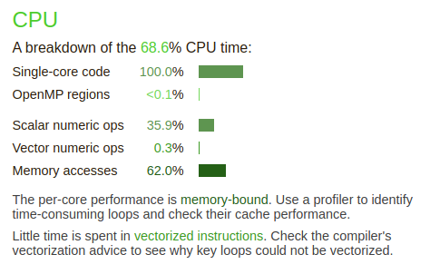
Fig. 4 - Performance report Details - CPU

The CPU details give us some hints about the actual CPU usage and the application instructions and memory access. This is a pure MPI application and each rank is single core, hence 100% single core.

36% of the compute time is spend executing scalar numeric operations, only 0.3% is spend executing vector operations. This is not good, as the AMD Rome processors have AVX2 vector instructions capable of 256 bits, 4 double or 8 single precision of floating point operations in one instruction. Using only scalar instructions mean that we are only exploiting 1/4 or 1/8th of the total compute capacity of the processor.

62% of the compute time is spent waiting for data to be moved to and from memory into the processor. This is normally due to a limitation of the memory bandwidth as is normally the case or poor programming with a lot of random memory accesses. Poor memory bandwidth is a common performance limitation. While the AMD Rome processors in Betzy show memory bandwidth in excess of 300 Gbytes per second this is far from enough to keep up with a processor running at 2500 MHz. Example, 300 Gbytes/s is 37 G double precision floats per second. A single core can do 4 double precision operations per vector unit per clock or 2.5 GHz*4 = 10 Gflops/s. Then there are two vector units per core and 128 cores in total. The cache helps in data can be reused in several calculations, but as the measurements show the bulk of time is spent waiting for memory.

The comments below clearly indicate this as the application is memory bound and very little time is spent in vectorised code.

Details - MPI

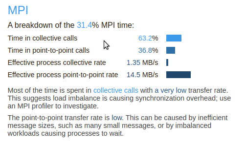
Fig. 5 - Performance report Details - MPI

The MPI details informs us that of the time spent in communication the majority of the MPI (63%) time is spent on doing collective operations, while the rest is spent in point-to-point communication. The relatively high fraction of time in collectives can be due to imbalance between the ranks. We see that the transfer rate is only in single digit Mbytes/s and only two digits for point-to-point. Very far from the wire speed at about 10 Gbytes/s.

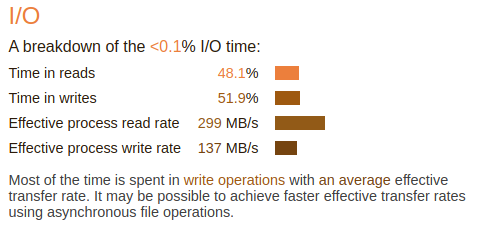
Fig. 6 - Performance report Details - IO

The IO details show that FVCOM spent a very little time doing IO during a run. About equal time for read and write. The transfer bandwidth is low as the file system is capable of far higher bandwidth.

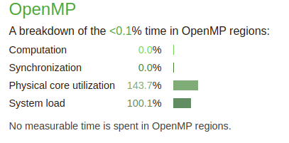
Fig. 7 - Performance report Details - OpenMP

The OpenMP (threads) detail report is of little use for FVCOM as it is a single threaded put MPI application. The same division as for MPI is relevant here computation and synchronisation. In OpenMP which used shared memory there is no transfer of data as all is in the same memory, but access control is very important. Hence synchronisation can make up a fraction of the time. False sharing is thing to look out for here when developing multi threaded programs. It’s easy to forget that while processor address individual bytes the cache is 64 bytes chunks of memory that might overlap with another thread in another core and cache line.

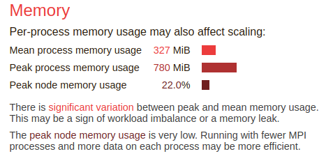
Fig. 8 - Performance report Details - Memory

The Memory detail report show the amount of memory used, mean and peak. As for FVCOM with the input model in question it uses only 22% of the nodes’ memory.

It does unfortunately not give any information about strided or random access. Even scalar operation can exhibit nice strided access. Any form of random access can kill any performance. Accessing bytes at 100 nm access time (for normal DDR memory) effectively run the processing speed at 10 MHz frequency.

Intel Advisor

Introduction

I order to get even more insight of your application with respect to code generated (vector instructions, vectorised loops etc), performance and memory access the tool Intel Advisor come in handy.

It’s very good for investigating how the compiler generated vector code and also providing hints about vectorisation. It can also provide information about memory access, like striding type.

It can record memory bandwidth and flops which is used to make a roof-line model. Please read about the roof-line model. if you are unfamiliar with it.

This case study does not go into depth on how to understand the advisor tool, this is far better covered in the Intel tools documentation, where they also provide a nice selection of tutorials.

Running and collecting

The GUI can be used to set up, launch, control and analyse the application. However, it’s simpler to collect data within a batch job. When running MPI jobs it’s only needed to run a single executable as they are all the same. A project directory need to be created before command line collection can be initiated.

The commands that used to collect data for FVCOM in the batch job are when using OpenMPI:

module load Advisor/2019_update5

advdir=$(dirname $(which advixe-cl))
mpirun -np 1  $advdir/advixe-cl -project-dir /cluster/work/support/olews/FVCOM_build/MATNOC-iompi/PO3/fvcom3   --collect survey -- ./fvcom.bin --casename=$RUN : -np 1023  ./fvcom.bin --casename=$RUN  > $RUN_DIR/log-${SLURM_JOBID}.out

An absolute path for mpirun arguments is needed, either full path or relative. The project directory is also given with full path. This directory need to be present before the collection begin.

When survey has been run tripcounts and flops can be collected.

module load Advisor/2019_update5

advdir=$(dirname $(which advixe-cl))
mpirun -np 1  $advdir/advixe-cl -project-dir /cluster/work/support/olews/FVCOM_build/MATNOC-iompi/PO3/fvcom3   --collect tripcounts -flop -- ./fvcom.bin --casename=$RUN : -np 1023  ./fvcom.bin --casename=$RUN  > $RUN_DIR/log-${SLURM_JOBID}.out

Memory access can be collected using the map keyword.

module load Advisor/2019_update5

advdir=$(dirname $(which advixe-cl))
mpirun -np 1  $advdir/advixe-cl -project-dir /cluster/work/support/olews/FVCOM_build/MATNOC-iompi/PO3/fvcom3   --collect map -flop -- ./fvcom.bin --casename=$RUN : -np 1023  ./fvcom.bin --casename=$RUN  > $RUN_DIR/log-${SLURM_JOBID}.out

Both tripcounts and map increase the run time significantly, remember to increase the Slurm run time.

Display Survey

To display the collected data please start the Advisor GUI tool using (remember to log in using ssh -Y, so the login nodes have connection to your X11 terminal):

advixe-gui &

Open the project file and report file on rank0 (we run the collection on rank0).

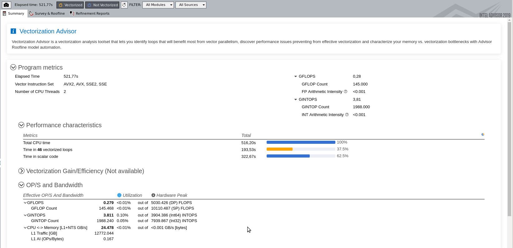
The fist screen show en overview of the run, elapsed time, time in vector and scalar code. In addition Gflops/s for Floating point & integer and some CPU cache data load. The fact that only 37.5% of the CPU time is spent executing vector instructions tells us that the compiler did not manage to vectorise the loops as often as we would hope for.

Display Roof-line model

By clicking at the vertical stripe marked “roofline” the obtained roof-line model of the application is displayed. It shows us graphically how the application map out on a memory bandwidth vs performance scale, see link to roof-line model above.

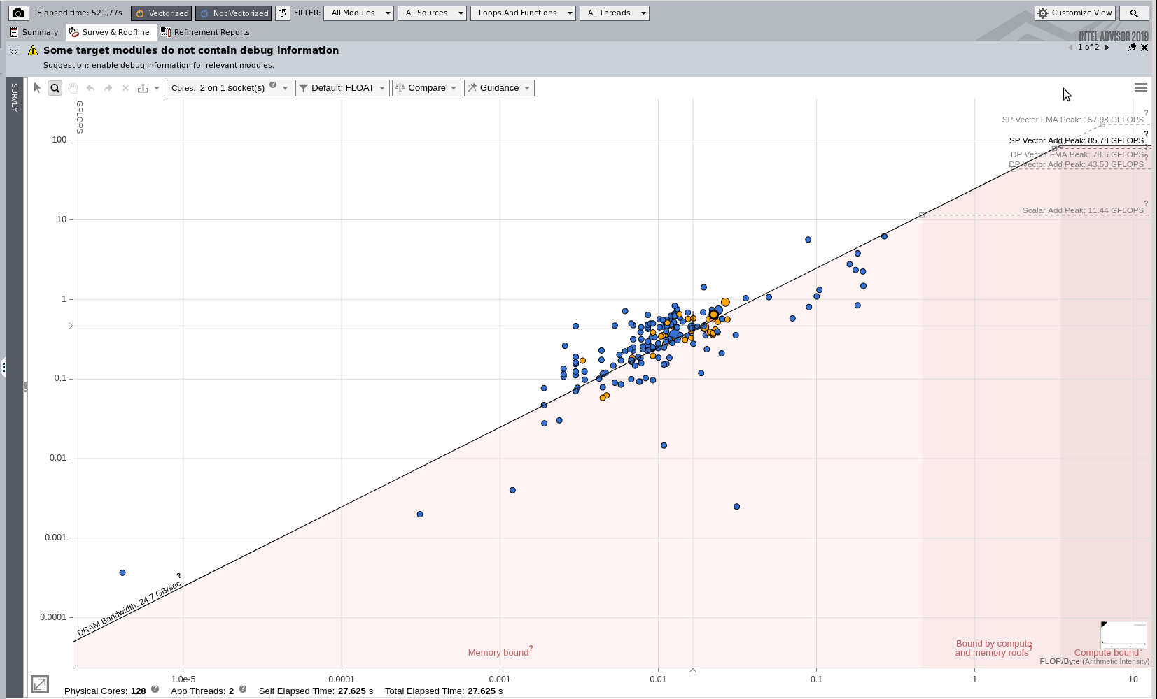
The circles are all located at the memory bandwidth line and left the regions where the application is compute bound. This is another illustration that the application performance is limited by the memory bandwidth. The two colours identifies scalar (blue) and vector (orange) performance.

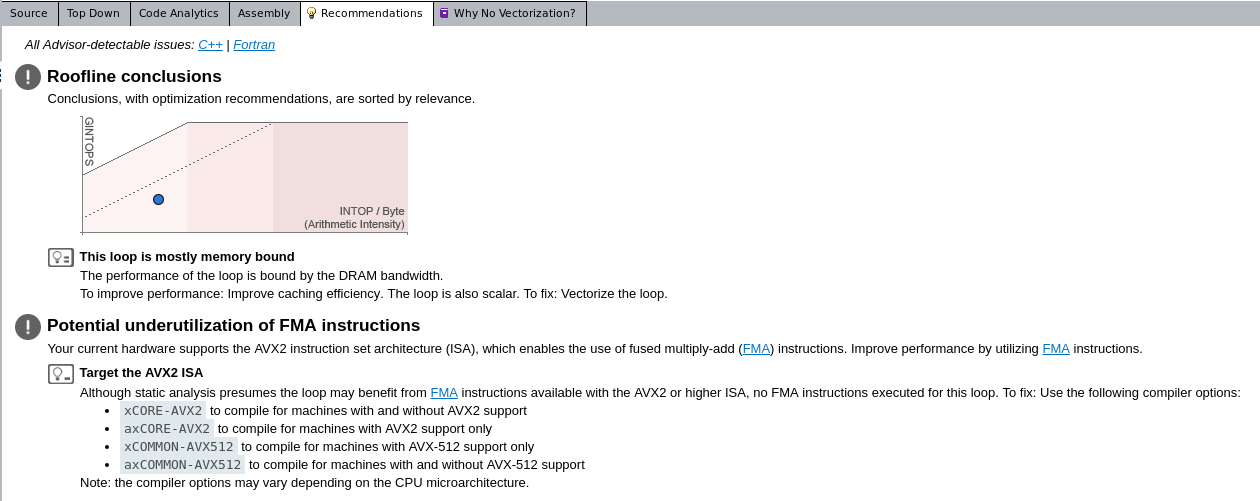
The Advisor can also generated some recommendations that can be helpful.

Display Memory access

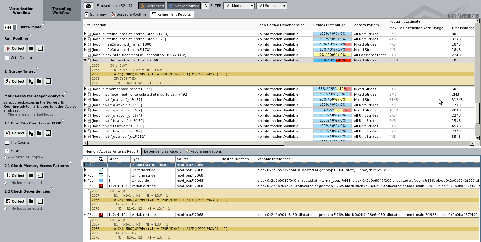
The map collection will record memory accesses and lump them into categories for unit, constant and variable stride. It’s well known that variable stride is very bad for performance. By providing references to the source code it’s possible to review the code and see if it’s possible to rewrite or do any changes that will improve performance.

Display memory dependencies

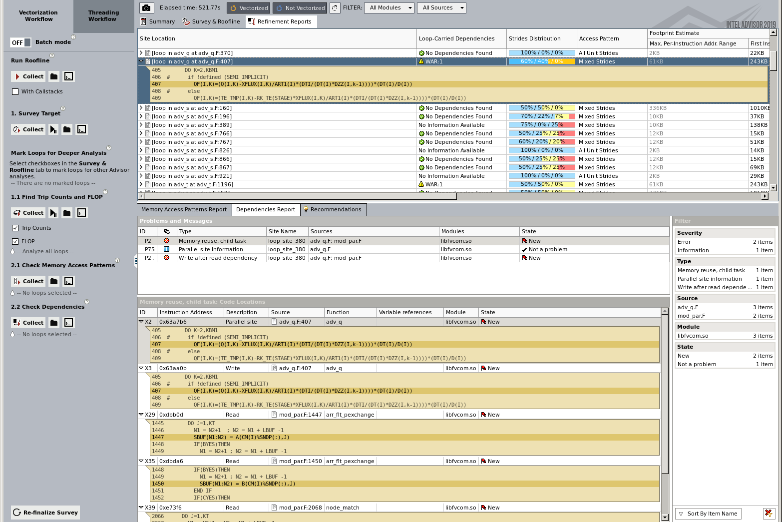
The dependency collection (takes very long time 20-100x normal run time) record variable that reuse same variables, e.g. memory location and potential race condition and sharing. The compiler need to take action and generate code that places locks and semaphores on such variables. This can have significant impact on performance.

Program efficiency

The Advisor can calculate a total performance of the complete run:

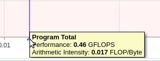
The number is discouraging, 0.46 Gflops/s. A single core can perform the following with two vector units at 256 bits each : 2.5 GHz * 256 bits (4 double,64 bits) * 2 (two vector units) = 20 Gflops/s or using Fuse multiply add to get twice the performance at 40 Gflops/s. For single precision 32 bits the numbers can be multiplied by two.

Using the most conservative numbers for double precision and not fused multiply add (20 Gflops/s) we get 0.46 / 20 = 2.3% of the theoretical performance.

This performance is not unusual for scientific code of this type. We saw early on that only a fraction of the time (68.6%) was spent in CPU time, of that time only a fraction was spent computing (35.9 + 0.3 = 36.2%). Combining this we arrive at 0.686*0.36.2=0.248 or 25% of the time was spent computing.