Introduction

Divide-n-conquer strategy is the foundation of parallel programming in which a bigger problem is divided into a set of smaller problems and solved efficiently. To design a generalized parallel programming model, which can fit a variety of problems, several methodologies were proposed around divide-n-conquer, and among them, one is Foster’s methodology. PCAM is the building block of Foster’s methodology, which stands for Partitioning, Communication, Agglomeration, and Mapping. Since the design and paradigm of parallel programming is a broad topic and beyond the scope of this tutorial, we will primarily focus on the Communication part of PCAM in this tutorial, and we shall see:

• What is a communication pattern in parallel computing

• A brief overview of Map and Gather communication patterns

• What are Stencil operation and its importance in numerical analysis

• Solving 2D heat equation using Stencil communication pattern in CUDA

• CUDA thread hierarchy

• Profiling our 2D heat equation code example

• How to Optimize our code example

• How to Debug our code example

Communication Patterns

What we know so far is that a parallel computation is divided into tasks, where each task is a unit of work. In CUDA, these tasks can be represented by CUDA threads. These threads need to work together and require inter-thread communication. In CUDA, communication happens through memory. For example, threads may need to read from an input memory location and write to the same memory location. Sometimes these threads exchange partial results with each other to compute the global result.

The communication between threads depends on the nature of the problem we wish to solve; For example, suppose the salary of ‘n’ employees in a company is stored in an array. Let us call this array ‘salary-array’. Now, we want to add a gift amount of 100 NOK to each employee’s salary. This task can be solved serially by iterating through the array, from the first to the last element in the array, and adding 100 NOK to each employee; clearly, this task will take ‘n’ steps to finish. The same task could have been solved parallelly in a constant time through the ‘MAP’ operation. MAP is a communication pattern where each thread reads and writes to a specific memory location, or we can say that there is a one-to-one correspondence between input and output. GPUs are very efficient in solving such problems, but Map is not very flexible in solving all types of computation problems; for example, Map cannot compute and store the average of 3 subsequent salaries of the employees in the array. However, another pattern called GATHER could solve the problem efficiently. In the case of Gather operation, each thread would read the values from 3 different locations in the memory and write them into a single place in the memory, as depicted in the figure.

Fig 1: MAP

Fig 2: GATHER

So far, we have seen that there are predefined communication patterns that appear now and again to solve a bigger problem, these patterns describe the basic solution to a problem and can be combined to solve a complex computational problem efficiently.

Stencil

Stencil operation computes the value of a single element by applying a function to a collection of neighboring elements. A very simple 9 elements stencil operation is shown in Fig 1. In one dimension, a nine-point stencil around a point at position \(x\) would apply some function to the values at these positions:

\[ {x − 4h, x − 3h, x − 2h, x − h, x, x + h, x + 2h, x + 3h, x + 4h}\]

Fig 3: Nine elements stencil.

As it can be seen from Fig 3 that 9 inputs are used to produce a single output. And if you look at our 9-point stencil operation again, then you will find that it is the finite-difference-method(FDM) of order 8 to calculate the first derivative of a function \({\displaystyle f(x)}\) at a point \(x\), and that is the reason why Stencil operation is at the core of many algorithms that solve partial differential equations.

2D Heat Equation

Heat dissipates into its surrounding by conduction, convection, and radiation. The process of transferring heat from the hotter part to the colder part of a material/body is called conduction. The heat equation models the flow of heat from the hotter part to the colder part of a body.

The heat equation is a fundamental differential equation because it is the building block for other differential equations and has applications across the sciences. Equation 1 is called the ideal heat equation because it models the heat flow in an ideal condition. For example, it does not consider the shape and type of the body. To apply it to real-world engineering problems, one should consider other physical constraints too.

(1)\[\begin{array}{cc}\frac{\delta u}{\delta t} = \alpha \left (\frac{\delta^2 u}{\delta y^2} + \frac{\delta^2 u}{\delta x^2} \right) \end{array}\]

If we try to solve Equation 1. We get:

(2)\[\begin{array}{cc} u_{ij}^{t+1} = u_{ij}^{t} + \Delta t\times\alpha \left( \frac{u_{i+1}^{t} + u_{i-1}^{t} + u_{j+1}^{t} +u_{j-1}^{t} -4u_{ij}^{t}}{h^2} \right) \end{array}\]

From Equation 2, we can see that the change in temperature after time \(\Delta t\) at a particular cell \(u_{ij}\) on the 2D surface, depends on its non-diagonal neighboring cells, as shown in Fig 4. You can also notice from Fig 4 that it is a 5-point stencil operation.

Fig 4: Discrete grid visualization.

Now, it is easy to translate Equation 2 into pseudocode.

Pseudocode for the heat flow on a 2D grid

for time 1 -> n :
    for cell(1,1) -> cel(grid_size, grid_size) :
         Temp_Next(i,j) = Temp_Cur(i,j) +
                          (
                           Temp_Cur(i+1,j) + Temp_Cur(i-1,j) +
                           Temp_Cur(i,j+1) + Temp_Cur(i,j-1) -
                           4.0 * Temp_Cur(i,j)
                          ) / Cell_Surface_Area

Neumann Boundary Condition

As we can see from Fig 4 that each cell needs 4 neighbor cells to calculate ‘Temp_Next’. But, what will happen at the corners and the edges of our grid? We will fall short of 2 cells at each corner-cell, and 1 cell at each edge-cell. To fix this problem, we will use Neumann Boundary Conditions which say that the temperature change is \(0\) or \(\left( \frac{\delta u}{\delta t} = 0 \right )\) at the boundary. To satisfy the boundary condition, we create a Halo around our grid and copy the temperature from the adjacent edge-cell to the adjacent halo-cell, as shown in Fig 6.

Fig 5: Halo around the grid.

Now, we have everything in place to draw a flow chart for the heat simulation in 2D.

Fig 6: 2D heat simulation.

A sequential version of 2D heat simulation

Here is how the 2D heat equation is implemented in C, and the highlighted lines show the main stencil operation. The complete code can be downloaded from the Resources section.

// Evolve the 'next' field from 'curr' with total grid size of (size + 2)^2,
// 'alpha' is the diffusion constant and 'dt' is the time derivative
void evolve(const float* curr, float* next, const int size, const float
	    cell_size, const float alpha, const float dt) {
#define CURR(i,j) curr[((i)+1)*(size+2)+(j)+1]
#define NEXT(i,j) next[((i)+1)*(size+2)+(j)+1]
  const float r = alpha*dt;
  for ( int i=0; i<size; i++ )
    for ( int j=0; j<size; j++ )
      NEXT(i,j) = CURR(i,j) + r * (
				   (CURR(i-1,j)+CURR(i+1,j)+CURR(i,j-1)+CURR(i,j+1)-4.0*CURR(i,j)) / (cell_size*cell_size)
				   ); 
}

Compilation and execution on Betzy

Follow these steps to compile and run the 2DHeatEquation project on Betzy.

1. Download tarball to your local client.

2. Upload it to your Betzy login

3. Uncompress it

4. Build it

5. Execute it

The output of our serial version of code should look something similar to this.

srun: job 371234 queued and waiting for resources
srun: job 371234 has been allocated resources
Solving heat equation for grid 500 x 500 with 1000 iterations
Used 0.509 seconds to evolve field
Average time per field update: 0.509 ms

It is also possible to visualize the output, as shown below.

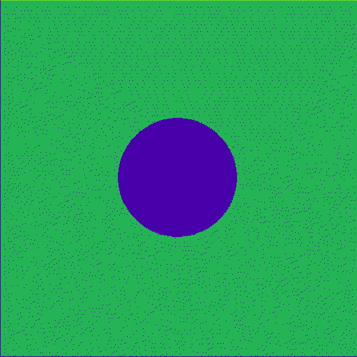
Fig 7: Heat diffusion in 2-dimension (Animation).

CUDA version of 2D heat simulation

Here is how the 2D heat equation is implemented in CUDA, and the highlighted lines show the main stencil operation. The complete code can be downloaded from the Resources section.

// Evolve the 'next' field from 'curr' with total grid size of (size + 2)^2,                                          
// 'alpha' is the diffusion constant and 'dt' is the time derivative                                                  
__global__ void evolve(const float* curr, float* next, const int size, const float
                       cell_size, const float alpha, const float dt) {
  const int i = blockIdx.x * blockDim.x + threadIdx.x;
  const int j = blockIdx.y * blockDim.y + threadIdx.y;
#define CURR(i,j) curr[((i)+1)*(size+2)+(j)+1]
#define NEXT(i,j) next[((i)+1)*(size+2)+(j)+1]
  // Additional variables                                                                                             
  const float cell = cell_size * cell_size;
  const float r = alpha * dt;                                                                                                
  if (0 < i && i < size + 1 && 0 < j && j < size + 1) {
    NEXT(i,j) = CURR(i,j) + r * (
                                 (CURR(i-1,j)+CURR(i+1,j)+
                                  CURR(i,j-1)+CURR(i,j+1)-
                                  4.0*CURR(i,j)) / (cell_size*cell_size)
                                 );
  }
}

Follow the instructions to Build and Run the CUDA code on Betzy.

The output of our CUDA code should look something similar to this.

Solving heat equation for grid 500 x 500 with 1000 iterations
Launching (32, 32) grids with (16, 16) blocks
Used 0.017 seconds to evolve field
Average time per field update: 0.017 ms

The code explanation is straightforward and very similar to the serial version. However, few new concepts have been introduced here, like Grid, Blocks, and Threads. We try to explain each of them briefly; however, an in-depth explanation is given on the Nvidia CUDA documentation page.

CUDA thread hierarchy

In a typical CUDA program, first, the CPU allocates storage on the GPU and copies the input data from the CPU to the GPU. The function which runs on a GPU is called a Kernel function or simply a Kernel. The CPU launches the Kernel, and the execution transfers from the CPU to the GPU. Input data get processed on the GPU and the results transfer back to the CPU.

During the execution of the Kernel, CUDA launches a large number of threads. To organize these threads, CUDA maintains a thread hierarchy. According to this 2-tier thread hierarchy, threads are divided into Blocks of threads, and blocks are divided into Grids of blocks, as shown in figure 8.

Fig 8: CUDA Grid, Blocks, and Threads.

A user has full control over organizing the threads into blocks and grids, and this can be done during the Kernel call; on the host side. An example of this is shown below.

Example of thread organization in Blocks and Grids.

 const dim3 blockSize(32,32);
 const dim3 gridSize(24,19);

 my_kernel<<<gridSize, blockSize>>>()

The above example shows that my_kernel will spawn 466,944 threads in total. To organize these many threads, the threads are organized into blocks of 32x32 threads in X and Y dimensions. So, each block has 32 threads in the X dimension, and 32 threads in the Y dimension; in total, each block has 1024 threads. Now the blocks are arranged in a grid of 24 blocks in the X dimension, and 19 blocks in the Y dimension; in total, 456 blocks in a grid.

Please note that dim3 is a derived data type wrapped around the intrinsic integer data type. It has three unsigned integers to store X, Y, and Z dimensions respectively.

The main purpose of this 2-tier hierarchy is to uniquely identify a thread in a pool of threads. Since thread blocks are spread across a 2-dimensional grid, it is easy to identify the block number, at run time, using variables supplied by CUDA-Runtime. Let us try to understand this with an example. Suppose, at a particular moment in time, we want to know the offset of our thread, then what should be our approach to find the global index of our thread?

Uniquely identify a thread within a pool of threads launched by a Kernel.

 /*
 CUDA-Runtime can provide these variables at runtime:
 ----------------------------------------------------
 1. gridDim.x
 2. gridDim.y
 3. blockIdx.x
 4. blockIdx.y
 5. threadIdx.x
 6. threadIdx.y
 */

 // Calculate the global thread index using these steps:

 // 1. Find the block number in which the current thread resides
 int global_block_index = gridDim.x*blockIdx.y + blockIdx.x;

 // If 1 block contains m*n threads then p blocks contain how many threads? p*m*n
 int total_threads = gloabal_block_index * blockDim.x*blockDim.y;

 // 3. Find the index of the current thread within the current block
 int local_thread_index = threadIdx.y*blockDim.x + threadIdx.x;

 // 4. Global thread index
 int global_thread_index =  total_threads + local_thread_index

 // One liner
 int offset = (gridDim.x*blockIdx.y + blockIdx.x)*(blockDim.x*blockDim.y)
              + threadIdx.y*blockDim.x + threadIdx.x;

 // Calculate global row and column of a thread
 int row = blockIdx.x * blockDim.x + threadIdx.x;
 int col = blockIdx.y * blockDim.y + threadIdx.y;

Designing the Cuda code

In this section, we will try to explain the sample Cuda code with the knowledge we got in the previous section.

In our Cuda code example, we used the Unified Memory feature of CUDA-6.0, and that is the reason why we did not allocate the memory using cudaMalloc, and also the data movement from host-to-device and device-to-host was not performed using cudaMemcpy; however, these two operations were taken care of by a unified function called cudaMallocManaged. This function allocates a unified pool of memory which is accessible both from the host and the device. Let us try to figure out where these operations were performed in our Cuda code.

In the following lines of code, you may see that after including some libraries and header files, we declared a few variables in line:77,78, like dim_block, and dim_grid. Here dim3 is a data type, provided by the CUDA-Runtime environment. The main use of this data type is to define the dimensions of a block and a grid. We kept the block size fixed with 256 threads in each block. The number of blocks in a grid is calculated in line:84. Please note that this number of blocks can only accommodate grid+2 elements, but our 2D grid has grid+2 x grid+2 elements, and that is the reason why we specified dim3(grids, grids) in line:85.

#include "png_writer.h"

#include <cuda.h>
#include <cuda_runtime_api.h>
#include <math.h>
#include <omp.h>
#include <stdio.h>
#include <stdlib.h>

// Default grid size (GRID_SIZE * GRID_SIZE elements are needed)
static const int DEFAULT_GRID_SIZE = 500;
// Default number of iterations if no command line argument is given
static const int DEFAULT_ITER = 1000;
// Default diffusion constant
static const float DEFAULT_ALPHA = 0.1;
static const float DEFAULT_CELL_SIZE = 0.01;
// Number of blocks to use when launching CUDA kernels
static const int FIXED_BLOCKS = 16;

// Forward declarations
// Initialize the field with a size of (size + 2)^2
__global__ void init_field(float* field, const int size);
// Evolve the 'next' field from 'curr' with total grid size of (size + 2)^2,
// 'alpha' is the diffusion constant and 'dt' is the time derivative
__global__ void evolve(const float* curr, float* next, const int size, const float cell_size, const float alpha, const float dt);
// Helper method to save the field to PNG
void save(const float* field, const int size, const int iteration);
// Check the return value of a CUDA function and abort if abnormal behavior
void check_cuda(const cudaError_t err, const char* msg);

int main(int argc, char* argv[]) {
  // grid_size represents the N x N grid to compute over
  int grid_size = DEFAULT_GRID_SIZE;
  // The number of iterations to perform to solve the equation
  int num_iter = DEFAULT_ITER;
  // Diffusion constant
  float alpha = DEFAULT_ALPHA;
  // Size of each grid cell
  float cell_size = DEFAULT_CELL_SIZE;
  // Calculate the time increment to propagate with
  const float dt = pow(cell_size, 4) / (2.0 * alpha * (pow(cell_size, 2) + pow(cell_size, 2)));
  // Save interval
  int save_interval = -1;

  // Command line handling
  if (argc > 1) {
    grid_size = atoi(argv[1]);
  }
  if (argc > 2) {
    num_iter = atoi(argv[2]);
  }
  if (argc > 3) {
    save_interval = atoi(argv[3]);
  }

  // Initialization
  printf("Solving heat equation for grid \033[0;35m%d x %d\033[0m with \033[0;35m%d\033[0m iterations\n",
    grid_size, grid_size, num_iter);
  // Setup CUDA block and grid dimensions to use for kernel launch
  dim3 dim_block;
  dim3 dim_grid;
  if (grid_size + 2 < 32) {
    dim_block = dim3(grid_size + 2, grid_size + 2);
    dim_grid = dim3(1, 1);
  } else {
    dim_block = dim3(FIXED_BLOCKS, FIXED_BLOCKS);
    const int grids = (grid_size + 2 + FIXED_BLOCKS - 1) / FIXED_BLOCKS;
    dim_grid = dim3(grids, grids);
  }
  printf("Launching \033[0;35m(%d, %d)\033[0m grids with \033[0;35m(%d, %d)\033[0m blocks\n",

In lines:90,91 we declared two pointers to deference the memory location, however, at this point in time no memory was allocated and therefore they are only null-pointers. lines:92,94 used the cudaMallocManaged function to allocate the unified memory space and map it to the pointers, which were declared in lines:90,91. Henceforth, all the modifications, in the allocated memory space, will be carried out using these pointers. In line:97 a device Kernel was launched which would calculate the initial and boundary conditions of the grid.

    dim_grid.x, dim_grid.y, dim_block.x, dim_block.y);
  // Setup grid arrays
  float* grid;
  float* next_grid;
  check_cuda(cudaMallocManaged(&grid, (grid_size + 2) * (grid_size + 2) * sizeof(float)),
    "Could not allocate 'grid'");
  check_cuda(cudaMallocManaged(&next_grid, (grid_size + 2) * (grid_size + 2) * sizeof(float)),
    "Could not allocate 'next_grid'");
  
  init_field<<<dim_grid, dim_block>>>(grid, grid_size);
  check_cuda(cudaGetLastError(), "'init_field' of 'grid' failed");
  init_field<<<dim_grid, dim_block>>>(next_grid, grid_size);
  check_cuda(cudaGetLastError(), "'init_field' of 'next_grid' failed");

The main stencil operation was performed in the evolve device kernel, which was run for the required number of iterations and timed using a time function. The logic behind the evolve function is similar to the serial version of the code, but in the Cuda version, evolve function is performed parallelly by Cuda threads. In line:122, system-level synchronization is used to make sure that the GPU and the CPU are synced; before any computed result is made available on the CPU. And lastly, the allocated memory is freed up in line:138,139.

  if (save_interval > 0) {
    check_cuda(cudaDeviceSynchronize(), "'init_field' of 'grid' or 'next_grid' failed");
    save(grid, grid_size, 0);
    if (grid_size < 34) {
      for(int i = 0; i < grid_size + 2; i++) {
	for(int j = 0; j < grid_size + 2; j++) {
	  const int index = i * (grid_size + 2) + j;
	  printf(" %2.0f", grid[index]);
	}
	printf("\n");
      }
    }
  }

  // Main calculation
  const double start_time = omp_get_wtime();
  for (int i = 1; i <= num_iter; i++) {
    // One iteration of the heat equation
    evolve<<<dim_grid, dim_block>>>(grid, next_grid, grid_size, cell_size, alpha, dt);
    // Wait until the kernel is done running before performing pointer swap
    check_cuda(cudaDeviceSynchronize(), "Waiting for evolve before pointer swap");
    // Exchange old grid with the new updated grid
    float* tmp = grid;
    grid = next_grid;
    next_grid = tmp;

    // Save image if necessary
    if (save_interval > 0 && (i % save_interval) == 0) {
      save(grid, grid_size, i);
    }
  }
  const double total_time = omp_get_wtime() - start_time;
  printf("Used \033[0;35m%.3f\033[0m seconds to evolve field\n", total_time);
  printf("Average time per field update: \033[0;35m%.3f\033[0m ms\n", (total_time * 1e3) / num_iter);

  // Free data and terminate
  cudaFree(grid);
  cudaFree(next_grid);
  return EXIT_SUCCESS;

Profiling

We will check our kernel performances using Nvidia Nsight Systems, which is a profiler and can be downloaded from Nvidia`s official website.

Profiling your Cuda code on Betzy or Saga is not difficult, but involves a few steps to follow. We will use nsys CLI to generate a view of our Cuda executable on the GPU cluster, and later analyze it on our local computer.

The basic qdrep file can be generated by following the command.

[@login-2.BETZY ~]$ module load CUDA/11.4.1
[@login-2.BETZY ~]$ cd HeatEq2D_Stencil/ 
[@login-2.BETZY ~]$ make clean
[@login-2.BETZY ~]$ make all
[@login-2.BETZY ~]$ srun --account=[USR-ACC] --time=05:00 --partition=accel --gpus=1 --mem-per-cpu=512M --job-name=nsys_stencil nsys profile -t cuda -f true -o cuda ./cuda

Detailed information about different nsys flags and options is provided here. But we use -t to profile cuda code, other options could be: openmp, mpi, openacc, nvtx, et cetera. Also, we used -f true to overwrite previously generated output, and -o to generate output in the folder ‘nvprofiler’ with the name ‘cuda’. Finally, we provided the executable name of our Cuda code. After executing the above command, we got output in the form of cuda.qdrep.

Now, download the ‘cuda.qdrep’ file to your local system using scp command, like this:

Note

Run this command on your local computer, and replace username with your user id and <absolute_path_to_the_file> with the path to the file on the cluster. pwd or readlink -f filename would help to know the absolute path of the file.

$ scp -r username@betzy.sigma2.no:<absolute_path_to_the_file> .

Now, launch the Nvidia Nsight Systems (I assume it has already been downloaded and installed on your local system). This should open a window similar to figure 9.

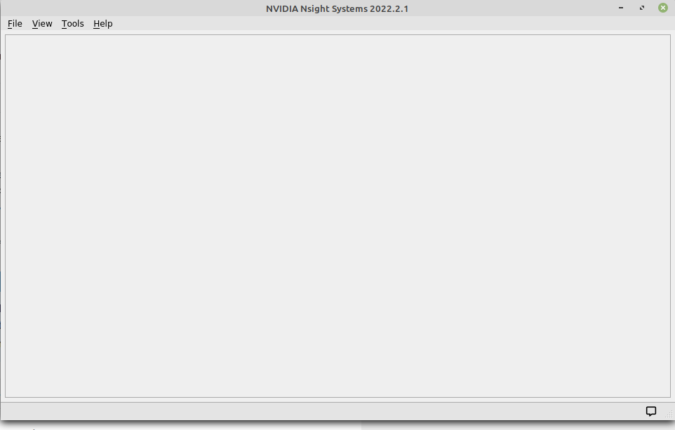
Fig 9: Nvidia Nsight Systems main window.

From the main menu, click ‘File’ and browse to the downloaded ‘cuda.qdrep’ file. This should open a ‘view’ similar to figure 10.

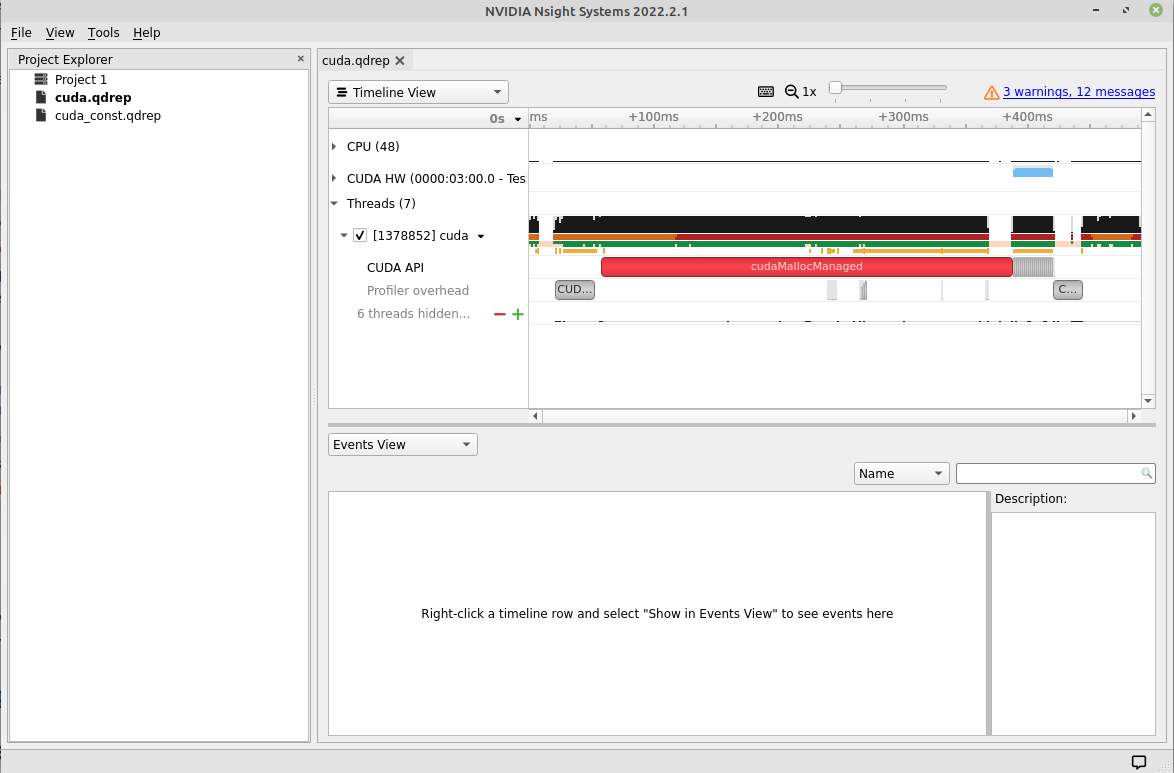
Fig 10: Main view window.

From the dropdown menu, one can choose Timeline, Analysis, or Diagnostic Summary. We are interested in the Timeline view, but some important information, like Target summary, Thread summary, and GPU-CPU info can be found in the ‘Analysis’ tab of this menu. As we can see from figure 10 that there are a few other collapsable tabs, like CPU(48), CUDA HW, etcetera. These tabs give information about the underlying resources our kernel used on the Target machine. If we click ‘CUDA HW’, then we see information about our kernels, as shown in figure 11.

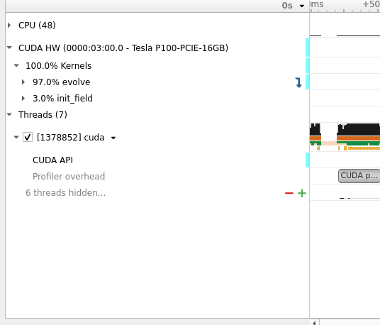
Fig 11: Executed kernels on the GPU.

This information is quite handy in knowing that our ‘evolve’ kernel has consumed 97% of the total kernel execution time on the GPU; apparently because the kernel has been called 1000 times, and init_field kernel called only 2 times for initializing the current and the next grid.

Now, if we look to the right of this tab, then we see the actual timeline, as shown in figure 12.

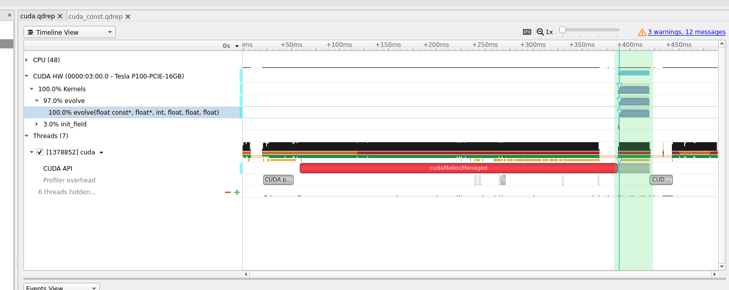
Fig 12: Actual timeline.

Drag the mouse cursor over the timeline during ‘evolve’ kernel execution time and press shift+z simultaneously to zoom in the timeline, as shown in figure 13. The figure shows that the kernel starts executing at around .389528s and ends at .389550s and took 22,688 microseconds to finish. This is the time utilization of a single kernel call, but we have called it 1000 times.

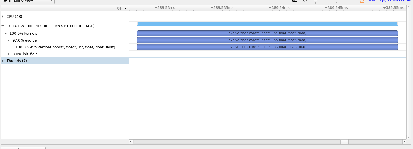
Fig 13: Zoomed timeline.

To analyze the complete summary, we must go to the bottom left pane of the main window in Nsight System, and select Stats System View from the dropdown list. This should show the relevant summary of our kernel call, as shown in figure 14. From the summary, we can see that most of the time was consumed by memory operations in moving data from host to device, and our ‘evolve’ kernel took around 22,516 microseconds on average.

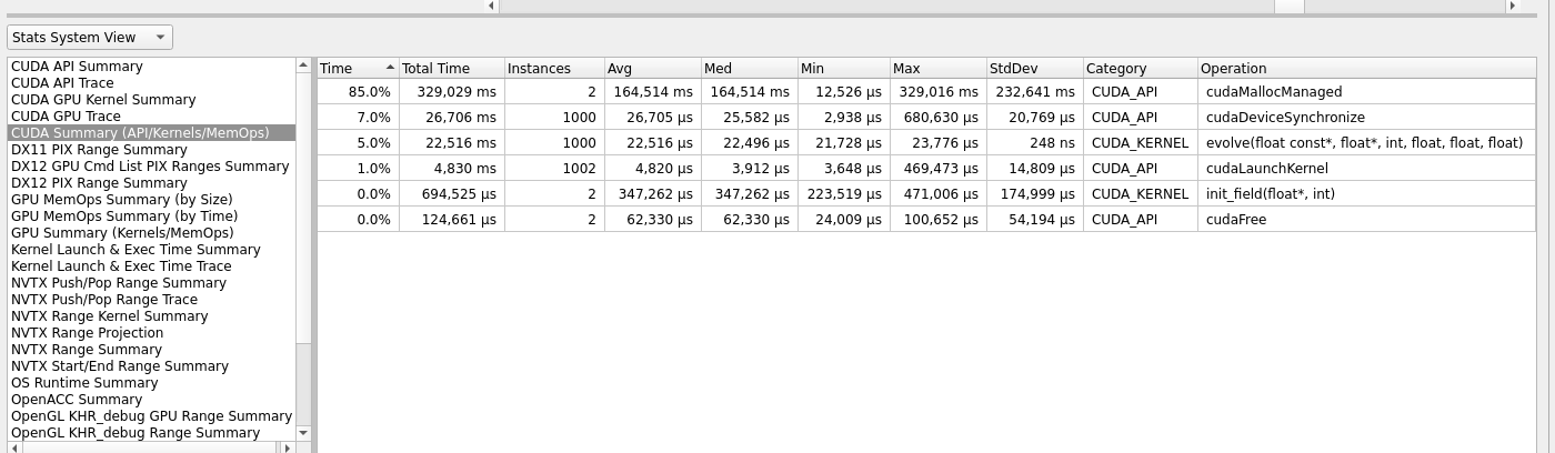
Fig 13: Summary of CUDA operations.

In the next section, we will try to reduce the total execution time by doing some memory optimization.

Optimization

In our Optimization section, we’ll try to incorporate onboard constant memory. Constant memory is only used for the reading purpose on the device and can be written or read from the host. The constant memory is accessible to all threads in a wrap, and each thread can access it uniformly.

Constant memory is located on the device and has its own on-chip cache, or we can say that each Streaming Multiprocessor has a constant cache. Because of this “per-SM” constant memory, reading takes less time as compared to reading directly from the constant memory.

The lifetime of a variable, which is declared and initialized on the constant memory, is equal to the lifetime of the program. A variable on the constant memory is accessible from any thread as long as the thread is from the same grid. The host can also read and write to the constant memory, but only through CUDA-Runtime functions. Variables on the constant memory must be pre-initialized before using them. Since the device code cannot write to the constant memory, the variables must be initialized from the host code using cudaMemcpyToSymbol, which is a CUDA-Runtime function.

Since our 2d-heat equation performs stencil operation which is a data-parallel operation and maps well to the GPU. Each thread calculates the change in temperature after a discrete time interval. During this calculation, each thread reads some constants, like the diffusion constant, time derivative etcetera. These constants tend to be the same throughout the execution of the program and would be a good candidate to use with constant memory.

To use the constant memory, we must setup it up from the host code, as shown in the code snippet. The highlighted line shows the copying of the data from the source to the constant memory on the device.

// constants array declaration using constant memory

__constant__ float constants[2]; // cell_size, alpha, dt

void setup_constants () {
  float cell_size = DEFAULT_CELL_SIZE;
  float alpha = DEFAULT_ALPHA;
  float dt = pow(cell_size, 4) / (2.0 * alpha * (pow(cell_size, 2) + pow(cell_size, 2)));
  float r = alpha * dt;
  const float host_constants[] = {cell_size, r};
  check_cuda(cudaMemcpyToSymbol(constants, host_constants, 2*sizeof(float)), "Error constant memory" );
}

Now, we must call the ‘setup_constants’ function before our ‘evolve’ kernel call, as shown here.

  // Main calculation
  setup_constants();
  const double start_time = omp_get_wtime();
  for (int i = 1; i <= num_iter; i++) {
    // One iteration of the heat equation
    // evolve<<<dim_grid, dim_block>>>(grid, next_grid, grid_size, cell_size, alpha, dt);
    evolve<<<dim_grid, dim_block>>>(grid, next_grid, grid_size);

Since we setup up our coefficients through constant memory, we do not need to send them as the function arguments during the kernel call.

The final thing remaining is to fetch the coefficients, on device, while doing computation. This can be done as shown below.

__global__ void evolve(const float* curr, float* next, const int size) {

  const int i = blockIdx.x * blockDim.x + threadIdx.x;
  const int j = blockIdx.y * blockDim.y + threadIdx.y;

  
#define CURR(i,j) curr[((i)+1)*(size+2)+(j)+1]
#define NEXT(i,j) next[((i)+1)*(size+2)+(j)+1]
  
  // Additional variables
  // const float cell = cell_size * cell_size;
  // const float r = alpha * dt;

  const float cell_size = constants[0];
  const float r = constants[1];

  // When launching this kernel we don't take into account that we don't want
  // it run for the boundary, we solve this by the following if guard, this
  // means that we launch 4 threads more than we actually need, but this is a
  // very low overhead

  if (0 < i && i < size + 1 && 0 < j && j < size + 1) {
    NEXT(i,j) = CURR(i,j) + r * (
                                 (CURR(i-1,j)+CURR(i+1,j)+
                                  CURR(i,j-1)+CURR(i,j+1)-
                                  4.0*CURR(i,j)) / (cell_size*cell_size)
                                 );
  }
  
}

// Helper method to save the field to PNG
void save(const float* field, const int size, const int iteration) {
  char filename[256];
  sprintf(filename, "field_%05d.png", iteration);

The complete source file can be downloaded from the given link.

cuda_const.cu

Let us re-run our code in the Nsight profiler.

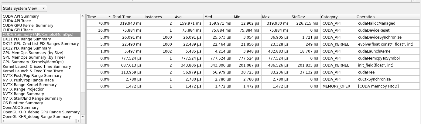
Fig 14: CUDA constant memory.

If we compare results from figure 13 and figure 14, we see that some improvement was achieved during data transfer, and little time reduction has been noticed in the evolve kernel execution.

Debugging

In this section, we will show some of the basic techniques to use CUDA gdb. CUDA gdb is an extension of the gdb debugger, which adds support for CUDA debugging. It supports breakpoints, single stepping, and everything else you would expect from a debugger. CUDA-gdb can be used to debug both the device code, as-well-as the host code.

To start the debugging session, we must provide the -G flag to our nvcc compiler. The -G flag enables debug symbols just like it would in the GNU-C compiler.

To make it a little fast and easy, I have included a CUDA-gdb enabled version of our 2DHeatequation code. You just need to compile and run it like this:

$ make cuda-gdb
cuda gdb code is built

$ srun --account=<UserAccount> --nodes=1 --ntasks-per-node=1 --time=05:00 --qos=devel --partition=preproc ./cuda-gdb
Submitted batch job 6990542

$ cat output.out
Waiting for evolve before pointer swap:
	Error(cudaErrorIllegalAddress): an illegal memory access was encountered

So, from the output, we know that illegal memory access has occurred somewhere in the code, with no other information. Luckily, we have CUDA-gdb to rescue us from this situation.

Since the code was compiled using proper flags to load debug symbols, we just need to invoke the CUDA-gdb, like this:

$ cuda-gdb ./cuda_gdb

The above command should start the gdb with command-line-interface, something similar to this:

NVIDIA (R) CUDA Debugger
11.1 release
Portions Copyright (C) 2007-2020 NVIDIA Corporation
GNU gdb (GDB) 8.3.1
Copyright (C) 2019 Free Software Foundation, Inc.
License GPLv3+: GNU GPL version 3 or later <http://gnu.org/licenses/gpl.html>
This is free software: you are free to change and redistribute it.
There is NO WARRANTY, to the extent permitted by law.
Type "show copying" and "show warranty" for details.
This GDB was configured as "x86_64-pc-linux-gnu".
Type "show configuration" for configuration details.
For bug reporting instructions, please see:
<http://www.gnu.org/software/gdb/bugs/>.
Find the GDB manual and other documentation resources online at:
    <http://www.gnu.org/software/gdb/documentation/>.

For help, type "help".
Type "apropos word" to search for commands related to "word"...
Reading symbols from ./cuda_gdb...
(cuda-gdb) 

Now, type run, this time we get a lot of vital information, and the execution would stop where it encountered the illegal memory access.

The information should look something similar to this:

(cuda-gdb) run
[Thread debugging using libthread_db enabled]
Using host libthread_db library "/lib64/libthread_db.so.1".
warning: File "/cluster/apps/eb/software/GCCcore/10.2.0/lib64/libstdc++.so.6.0.28-gdb.py" auto-loading has been declined by your `auto-load safe-path' set to "$debugdir:$datadir/auto-load".
To enable execution of this file add
	add-auto-load-safe-path /cluster/apps/eb/software/GCCcore/10.2.0/lib64/libstdc++.so.6.0.28-gdb.py
line to your configuration file "/cluster/home/user/.cuda-gdbinit".
To completely disable this security protection add
	set auto-load safe-path /
line to your configuration file "/cluster/home/user/.cuda-gdbinit".
For more information about this security protection see the
"Auto-loading safe path" section in the GDB manual.  E.g., run from the shell:
	info "(gdb)Auto-loading safe path"
Solving heat equation for grid 500 x 500 with 1000 iterations
Launching (32, 32) grids with (16, 16) blocks
[Detaching after fork from child process 1561068]
[New Thread 0x7fffef646000 (LWP 1561074)]
[New Thread 0x7fffeee45000 (LWP 1561075)]

CUDA Exception: Warp Illegal Address
The exception was triggered at PC 0x906110 (cuda_gdb.cu:209)

Thread 1 "cuda_gdb" received signal CUDA_EXCEPTION_14, Warp Illegal Address.
[Switching focus to CUDA kernel 0, grid 3, block (0,0,0), thread (1,1,0), device 0, sm 0, warp 1, lane 17]
0x0000000000906118 in evolve<<<(32,32,1),(16,16,1)>>> (curr=0x7fffbc000000, next=0x7fffbc0f6200, size=500, 
    cell_size=0.00999999978, alpha=0.100000001, dt=0.000249999983) at src/cuda_gdb.cu:209

Now, we know that the kernel ‘evolve’ is doing some illegal memory accesses. List the code around line number 209. We chose 209 because it is pointed out by the debugger. Since our listsize is set to 30, we would list the code from line number 200.

(cuda-gdb) list 200
185	
186	#define CURR(i,j) curr[((i)-1)*(size)+(j)-1]
187	#define NEXT(i,j) next[((i))*(size+2)+(j)]
188	
189	  
190	  // Additional variables
191	  const float cell = cell_size * cell_size;
192	  const float r = alpha * dt;
193	  // When launching this kernel we don't take into account that we don't want
194	  // it run for the boundary, we solve this by the following if guard, this
195	  // means that we launch 4 threads more than we actually need, but this is a
196	  // very low overhead
197	  /*
198	  if (0 < row && row < size + 1 && 0 < col && col < size + 1) {
199	    const int ip1 = (row + 1) * (size + 2) + col;
200	    const int im1 = (row - 1) * (size + 2) + col;
201	    const int jp1 = row * (size + 2) + (col + 1);
202	    const int jm1 = row * (size + 2) + (col - 1);
203	    next[index] = curr[index] + r *
204	      ((curr[ip1] - 2. * curr[index] + curr[im1]) / cell
205	      + (curr[jp1] - 2. * curr[index] + curr[jm1]) / cell) ;
206	  }*/
207	
208	  if (0 < i && i < size + 1 && 0 < j && j < size + 1) {
209	    NEXT(i,j) = CURR(i,j) + r * (
210	                                 (CURR(i-1,j)+CURR(i+1,j)+
211	                                  CURR(i,j-1)+CURR(i,j+1)-
212	                                  4.0*CURR(i,j)) / (cell_size*cell_size)
213	                                 );
214	  }

We can see that there are some reads and writes in line number 209. We can also see that some macro functions perform read operations. Let us test which memory address they are reading from.

(cuda-gdb) p i
$1 = 1
(cuda-gdb) p j
$2 = 1
(cuda-gdb) p curr[((i-1)-1)*(size)+(j)-1]
Error: Failed to read generic memory at address 0x7fffbbfff830 on device 0 sm 0 warp 1 lane 17, error=CUDBG_ERROR_INVALID_MEMORY_SEGMENT(0x7).

We are trying to read the memory past the lower bound of our allocated memory space on the device and thus get the error. Fix this by replacing 1 with 2.

1. #define CURR(i,j) curr[((i)-1)*(size)+(j)-1]
 
2. #define CURR(i,j) curr[((i))*(size)+(j)]

Resources

The complete code is available in compressed format and can be downloaded from the given link.

HeatEq2D_Stencil

Upload it to Betzy

$ scp <source_directory/HeatEq2D_Stencil.tar.gz> username@betzy.sigma2.no:/cluster/home/<target_directory>

Uncompress it on Betzy

$ tar -zxvf HeatEq2D_Stencil.tar.gz

Build project on Betzy

Build Serial version.

$ make serial

Build Parallel version.

$ make parallel

Note

Module CUDA/11.4.1 is required on Betzy to build GPU version.

Build CUDA version.

$ make cuda

Build complete project.

$ make all

Execute code on Betzy

Run Serial version.

$ srun --account=<UserAccount> --nodes=1 --ntasks-per-node=1 --time=05:00 --qos=devel --partition=preproc ./serial

Run Parallel version.

$ srun --account=<UserAccount> --nodes=1 --ntasks-per-node=1 --cpus-per-task=32 -c 32 --time=05:00 --mem-per-cpu=512M --qos=devel --partition=preproc ./parallel 

Run CUDA version.

$ srun --account=<User-Account> --partition=accel --gpus-per-task=1 --ntasks=1 --time=05:00 --mem-per-cpu=512M  ./cuda

Visualization on Betzy

$ srun --account=<UserAccount> --cpus-per-task=1 -c 1 --time=10:00 --mem-per-cpu=1G --qos=devel --partition=preproc ./serial 500 1000 2

The above command will generate one png file at every other iteration, and then you can use ffmpeg to create animation.