Profiling GPU-accelerated Deep Learning

We present an introduction to profiling GPU-accelerated Deep Learning (DL) models using PyTorch Profiler. Profiling is a necessary step in code development, as it permits identifying bottlenecks in an application. This in turn helps optimize applications, thus improving performance.

This introduction is limited to profiling DL-application that runs on a single GPU. By the end of this guide, readers are expected to learn about:

• Defining the concept and the architecture of PyTorch Profiler.

• Setting up PyTorch profiler on an HPC system.

• Profiling a PyTorch-based application.

• Visualizing the output data on a web browser with the Tensorboard plugin, in particular, the metrics:

  • GPU usage

  • GPU Kernel view

  • Memory view

  • Trace view

  • Module view

What is PyTorch Profiler

In general, the concept of profiling is based on statistical sampling, by collecting data at a regular time interval. Here, a profiler tool offers an overview of the execution time attributed to the instructions of a program. In particular, it provides the execution time for each function; in addition to how many times each function has been called. Profiling analysis helps to understand the structure of a code, and more importantly, it helps to identify bottlenecks in an application. Examples of bottlenecks might be related to memory usage and/or identifying functions/libraries that use the majority of the computing time.

PyTorch Profiler is a profiling tool for analyzing Deep Learning models, which is based on collecting performance metrics during training and inference. The profiler is built inside the PyTorch API (cf. Fig 1), and thus there is no need for installing additional packages. It is a dynamic tool as it is based on gathering statistical data during the running procedure of a training model.

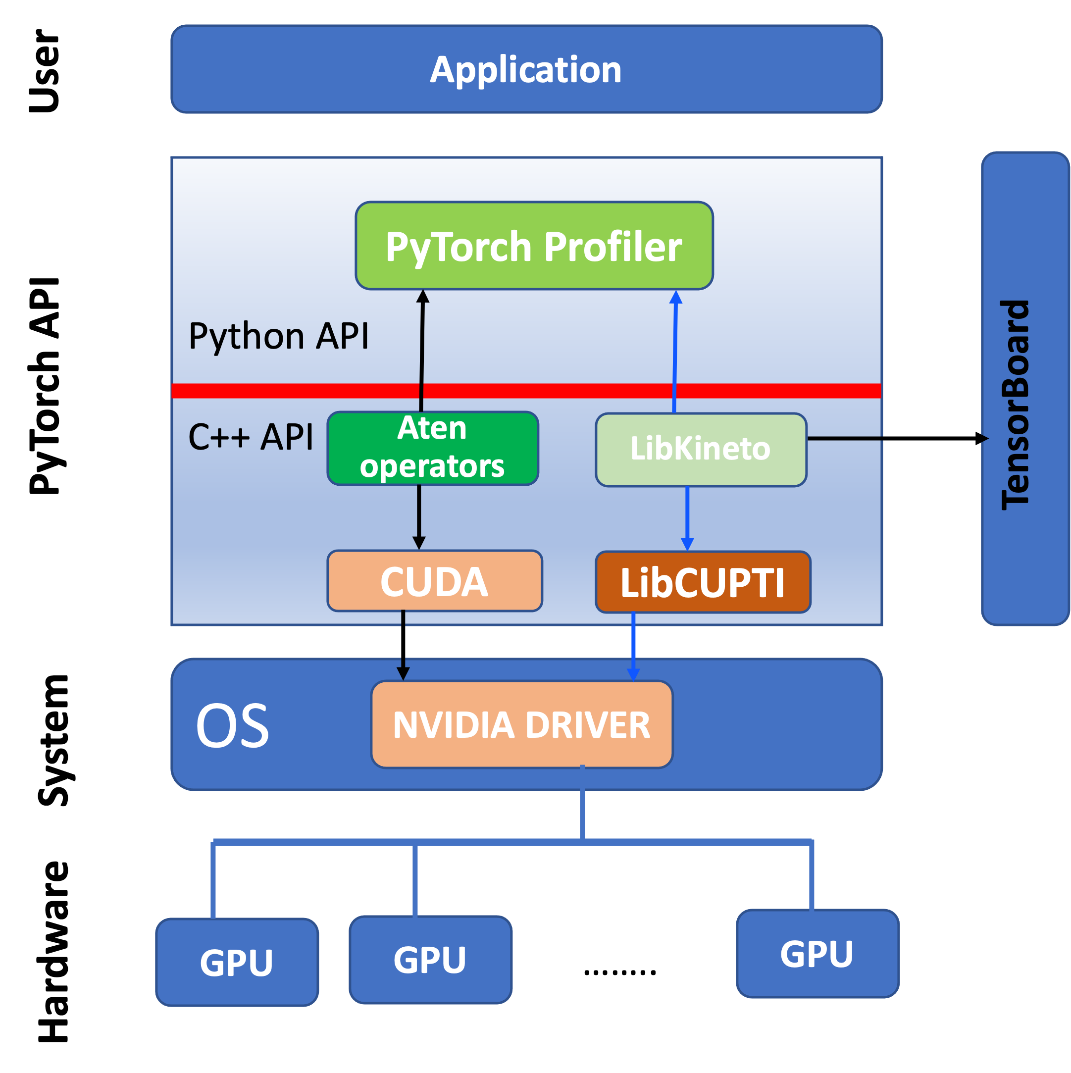
Fig 1: A simplified version of the architecture of PyTorch Profiler. A complete picture of the architecture can be found [here](#https://www.youtube.com/watch?v=m6ouC0XMYnc&ab_channel=PyTorch) (see the slide at 23:00 min).

As shown in the figure, the PyTorch API contains a Python API and a C++ API. For simplicity we highlight only the necessary components for understanding the functionality of PyTorch profiler, which integrates the following: (i) aTen operators, which are libraries of tensor operators for PyTorch and are GPU-accelerated with CUDA; (ii) Kineto library designed specifically for profiling and tracing PyTorch models; and (iii) LibCUPTI (CUDA Profiling Tool Interface), which is a library that provides an interface for profiling and tracing CUDA-based application (low-level profiling). The last two libraries provide an interface for collecting and analyzing the performance data at the level of GPU.

Here we list the performance metrics provided by the profiler, which we shall describe in Section:

• GPU usage

• Tensor cores usage (if it is enabled)

• GPU Kernel view

• Memory view

• Trace view

• Module view

Further details are provided in these slides.

Setup Pytorch profiler in an HPC system

In this section, we describe how to set up PyTorch using a singularity container.

• Step 1: Pull and convert a docker image to a singularity image format: e.g. from the NVIDIA NGC container

Note that when pulling docker containers using singularity, the conversion can be quite heavy and the singularity cache directory in $HOME space becomes full of temporary files. To speed up the conversion and avoid storing temporary files, one can first run these lines:

$ mkdir -p /tmp/$USER 
$ export SINGULARITY_TMPDIR=/tmp/$USER 
$ export SINGULARITY_CACHEDIR=/tmp/$USER

and then pull the container

$singularity pull docker://nvcr.io/nvidia/pytorch:22.12-py3

• Step 2: Launch the singularity container

$singularity exec --nv -B ${MyEx} pytorch_22.12-py3.sif python ${MyEx}/resnet18_api.py

Here the container is mounted to the path ${MyEx}, where the Python application is located. An example of a Slurm script that launches a singularity container is provided in the Section.

Case example: Profiling a Resnet 18 model

We consider the Resnet 18 model as an example to illustarte profiling with PyTorch profiler. Here we list the lines of code required to enable profiling with PyTorch Profiler

with torch.profiler.profile(
    activities=[
        torch.profiler.ProfilerActivity.CPU,
        torch.profiler.ProfilerActivity.CUDA],
    schedule=torch.profiler.schedule(
        wait=1,
        warmup=1,
        active=2),
    on_trace_ready=torch.profiler.tensorboard_trace_handler(‘./out', worker_name=‘profiler'),
    record_shapes=True,
    profile_memory=True, 
    with_stack=True
) as prof:

To be incorporated just above the training loop

#training step for each batch of input data
    for step, data in enumerate(trainloader):
          .
          .
          .
          .
       if step +1>= 10:
            break
        prof.step()

Here is a code example of the Resnet18 model, in which profiling is enabled. The code is adapted from the PyTorch tutorial.

#import all the necessary libraries 
import torch
import torch.nn
import torch.optim
import torch.profiler
import torch.utils.data
import torchvision.datasets
import torchvision.models
import torchvision.transforms as T
from torchvision.models import ResNet18_Weights

#prepare input data and transform it
transform = T.Compose([T.Resize(256), T.CenterCrop(224), T.ToTensor(), 
    T.Normalize((0.5, 0.5, 0.5), (0.5, 0.5, 0.5))])

#trainset = torchvision.datasets.CIFAR10(root='./data', train=True,transform=transform)
trainset = torchvision.datasets.CIFAR10(root='./data', train=True, 
    download=True, transform=transform)

# use dataloader to launch each batch
#trainloader = torch.utils.data.DataLoader(trainset, batch_size=1,shuffle=True, num_workers=4)
trainloader = torch.utils.data.DataLoader(trainset, batch_size=4,shuffle=True, num_workers=1)

# Create a Resnet model, loss function, and optimizer objects. To run on GPU, move model and loss to a GPU device
device = torch.device("cuda:0")

#model = torchvision.models.resnet18(pretrained=True).cuda(device)
model = torchvision.models.resnet18(weights=ResNet18_Weights.DEFAULT).cuda(device)
criterion = torch.nn.CrossEntropyLoss().cuda(device)
optimizer = torch.optim.SGD(model.parameters(), lr=0.001, momentum=0.9)
model.train()

#Use profiler
with torch.profiler.profile(
    activities=[
        torch.profiler.ProfilerActivity.CPU,
        torch.profiler.ProfilerActivity.CUDA],
    schedule=torch.profiler.schedule(
        wait=1,
        warmup=1,
        active=2),
    on_trace_ready=torch.profiler.tensorboard_trace_handler('./out', worker_name='worker4'),
    record_shapes=True,
    profile_memory=True,  # This will take 1 to 2 minutes. Setting it to False could greatly speedup.
    with_stack=True
) as prof:
#include
    for step, data in enumerate(trainloader):
        print("step:{}".format(step))
        inputs, labels = data[0].to(device=device), data[1].to(device=device)

        outputs = model(inputs)
        loss = criterion(outputs, labels)
        optimizer.zero_grad()
        loss.backward()
        optimizer.step()
        if step >= 10:
            break
        prof.step()

print()
print(f'--Print GPU: {torch.cuda.device_count()}')
print(torch.cuda.is_available())

For reference, we provide here the same application but without enabling profiling. The code is adapted from the PyTorch tutorial.

#import all the necessary libraries 
import torch
import torch.nn
import torch.optim
import torch.profiler
import torch.utils.data
import torchvision.datasets
import torchvision.models
import torchvision.transforms as T
from torchvision.models import ResNet18_Weights

#prepare input data and transform it
transform = T.Compose([T.Resize(256), T.CenterCrop(224), T.ToTensor(), 
    T.Normalize((0.5, 0.5, 0.5), (0.5, 0.5, 0.5))])

#trainset = torchvision.datasets.CIFAR10(root='./data', train=True,transform=transform)
trainset = torchvision.datasets.CIFAR10(root='./data', train=True, 
    download=True, transform=transform)

# use dataloader to launch each batch
#trainloader = torch.utils.data.DataLoader(trainset, batch_size=1,shuffle=True, num_workers=4)
trainloader = torch.utils.data.DataLoader(trainset, batch_size=4,shuffle=True, num_workers=1)

# Create a Resnet model, loss function, and optimizer objects. To run on GPU, move model and loss to a GPU device
device = torch.device("cuda:0")

#model = torchvision.models.resnet18(pretrained=True).cuda(device)
model = torchvision.models.resnet18(weights=ResNet18_Weights.DEFAULT).cuda(device)
criterion = torch.nn.CrossEntropyLoss().cuda(device)
optimizer = torch.optim.SGD(model.parameters(), lr=0.001, momentum=0.9)
model.train()

#Define the training step for each batch of input data.
def train(data):
    inputs, labels = data[0].to(device=device), data[1].to(device=device)
    outputs = model(inputs)
    loss = criterion(outputs, labels)
    optimizer.zero_grad()
    loss.backward()
    optimizer.step()

print()
print(f'--Print GPU: {torch.cuda.device_count()}')
print(torch.cuda.is_available())

In the lines of code defined above, one needs to specify the setting for profiling. The latter can be split into three main parts:

• Import torch.profiler

• Specify the profiler context: i.e. which kind of activities one can profile. e.g. CPU activities (i.e. torch.profiler.ProfilerActivity.CPU), GPU activities (i.e. torch.profiler.ProfilerActivity.CUDA) or both activities.

• Define the schedule; in particular, the following options can be specified: —wait=l: Profiling is disabled for the first l steps. This is relevant if the training takes a longer time, and that profiling the entire training loop is not desired. Here, one can wait for l steps before the profiling gets started.

  —warmup=N: The profiler collects data after N steps for tracing.

  —active=M: Events will be recorded for tracing during the active steps. This is useful to avoid tracing a lot of events, which might cause issues with loading the data.

• Additional options: Trace, record shape, profile memory, with stack, could be enabled.

Note that, in the for loop (i.e. the training loop), one needs to call the profile step (prof.step()), in order to collect all the necessary inputs, which in turn will generate data that can be viewed with the Tensorboard plugin. In the end, the output of profiling will be saved in the /out directory.

Note that a good practice of profiling should be based on the following: first one can start profiling for a large training loop, and once we identify the bottleneck, then we can select a few iterations for re-profiling and tuning the application. This should be followed by optimising the application and eventually re-profiling to check the impact of the optimisation.

Visualization on a web browser

To view the output data generated from the profiling process, one needs to install TensorBord. This can be done for instance in a virtual environment. Here we desccribe a step-by-step guide of the installation:

• Step 1: Load a Python model, create and activate a virtual environment. Load a Python module. e.g.: module load python/3.9.6-GCCcore-11.2.0`

• mkdir Myenv

• python –m venv Myenv

• source Myenv/bin/activate

• Step 2: Install TensorBoard Plugin via pip wheel packages using the following command (see also here):

• python –m pip install torch_tb_profiler

• Step 3: Run Tensorboard using the command:

tensorboard --logdir=./out --bind_all

This will generate a local address having a specific registered or private port, as shown in Figure. Note that in HPC systems, direct navigation to the generated address is blocked by firewalls. Therefore, connecting to an internal network from outside can be done via a mechanism called local port forwarding. As stated in the SSH documentation “Local forwarding is used to forward a port from the client machine to the server machine”.

The syntax for local forwarding, which is configured using the option –L, can be written as, e.g.:

ssh -L 6009:localhost:6006 username@server.address.com

This syntax enables opening a connection to the jump server username@server.address.com, and forwarding any connection from port 6009 on the local machine to port 6006 on the server username@server.address.com.

Lastly, the local address http://localhost:6009/ can be viewed in a Chrome or Firefox browser.

On Saga cluster

Here is an example about viewing data using TensorBoard on Saga. We assume that TensorBoard plugin is installed in a virtual environment, which we name Myenv as described above. Here are main steps:

Step 1: Source the virtual environment

$source Myenv/bin/activate

Step 2: Run the tensorboard command

$tensorboard --logdir=./out --bind_all`

Note that the profiled data are stored in the out folder. Running the command prints out a message that includes

...
...
$TensorBoard 2.13.0 at http://login-3.saga.sigma2.no:6006/
...

The output message contains the address of the current login node, which is in our case login-3.saga.sigma2.no. This address will be used as a jump server as expressed in the next step.

Step 3: In a new terminal, run this command

ssh -L 6009:localhost:6006 username@login-3.saga.sigma2.no

Note that the port number 6006 is taken form the address login-3.saga.sigma2.no:6006.

Step 4: View the profiled data in a Chrome or Firefox browser

http://localhost:6009/

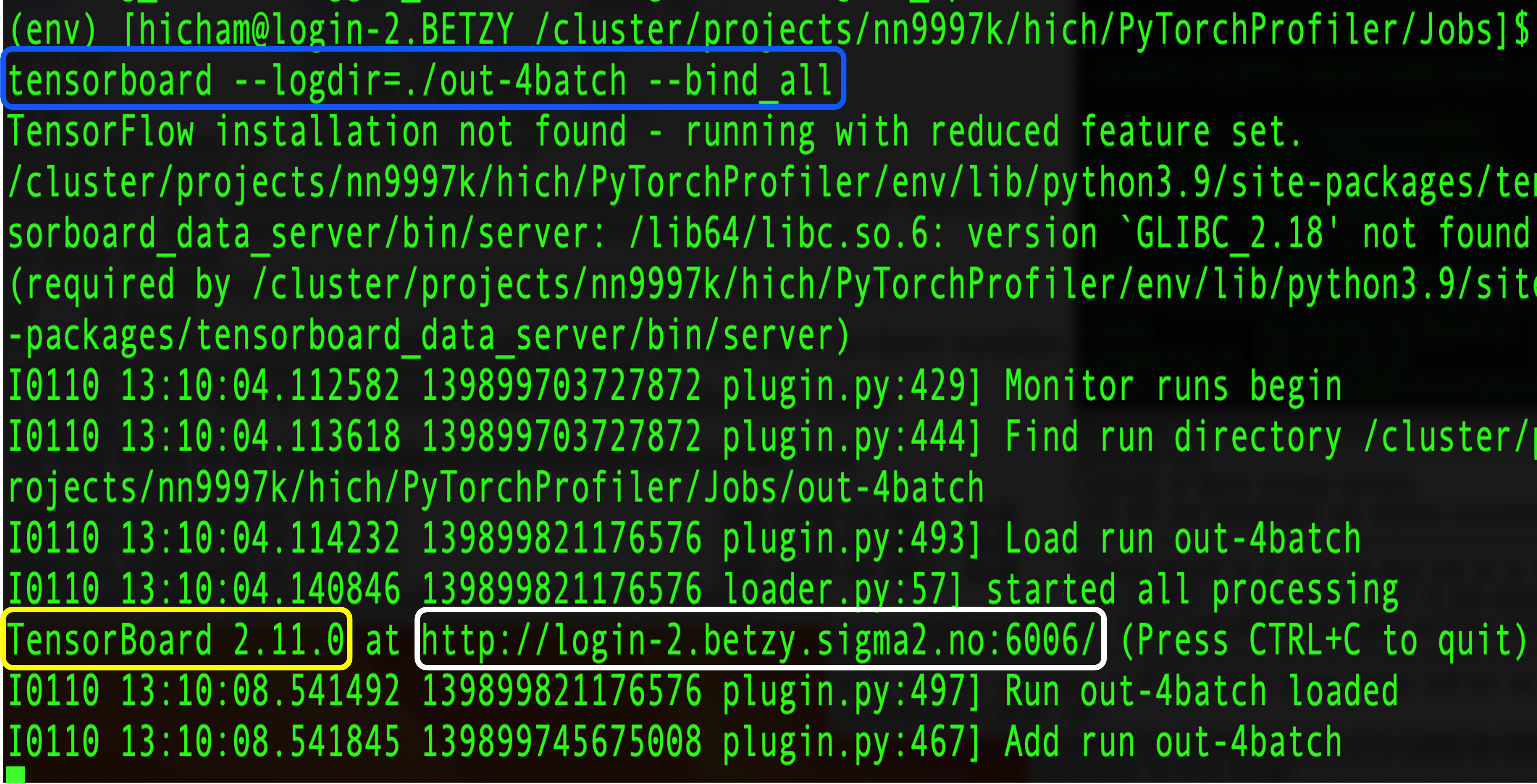
Fig 2: Output of running the tensorboar command tensorboard –logdir=./out –bind_all.

Performance metrics

In this section, we provide screenshots of different views of performance metrics stemming from PyTorch Profiler. The metrics include:

• GPU usage (cf. Figure 3)

• GPU Kernel view (cf. Figure 4)

• Trace view (cf. Figure 5 and Figure 6)

• Memory view (cf. Figure 7)

• Module view (cf. Figure 8)

Fig 3: Overview of GPU activities.

Fig 4: View of GPU Kernels.

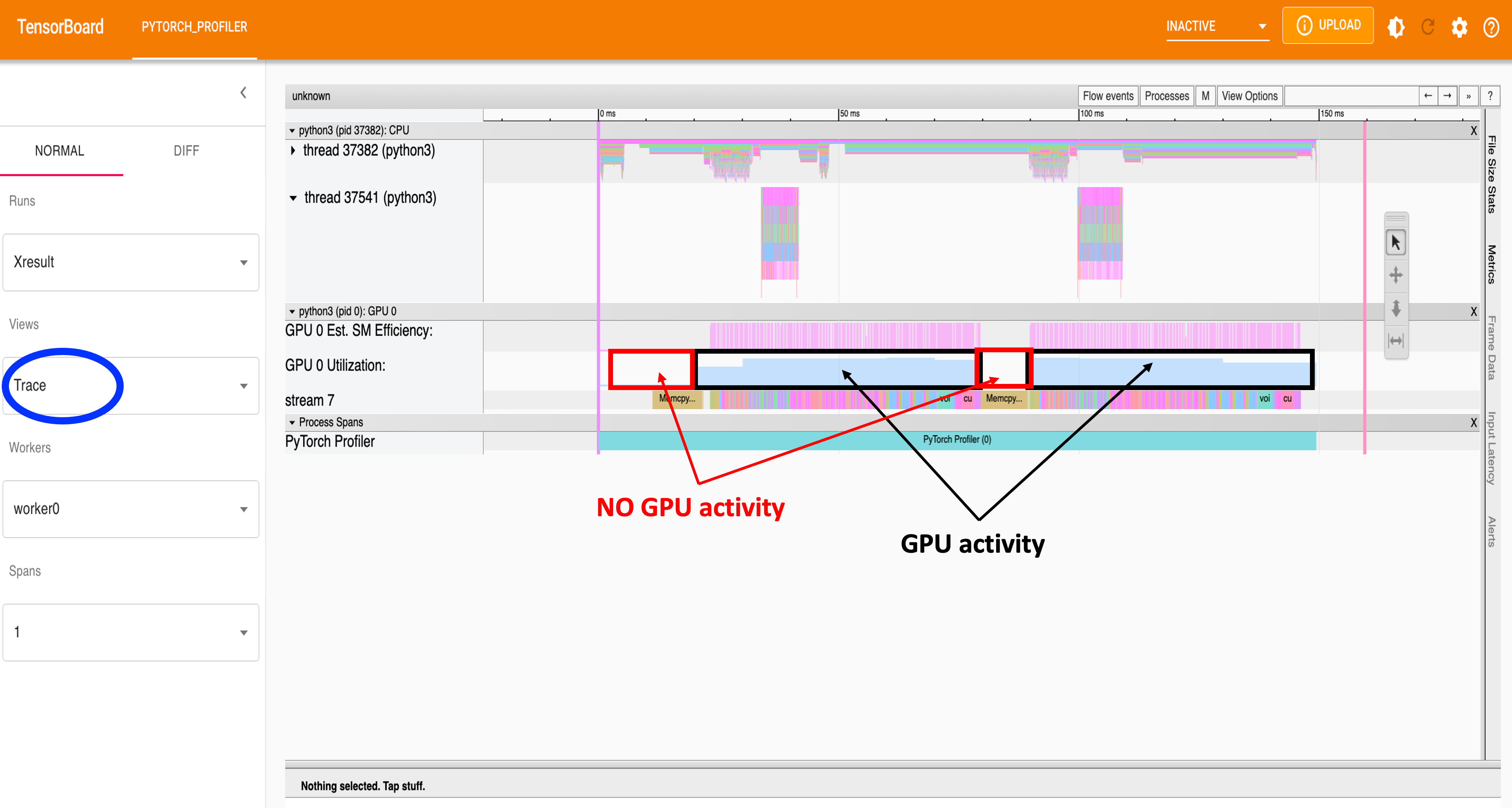
Fig 5: View of Trace.

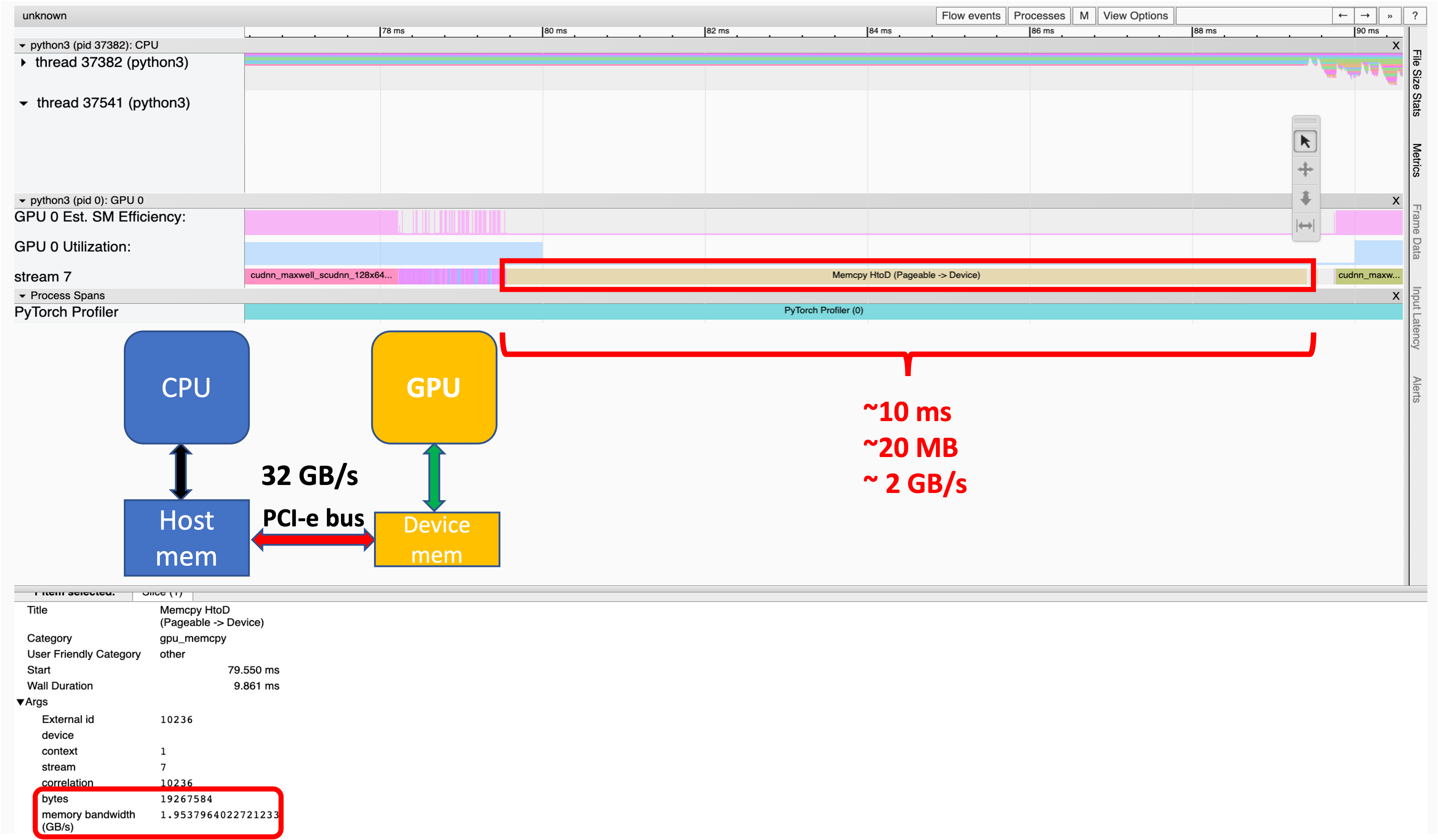
Fig 6: View of Trace.

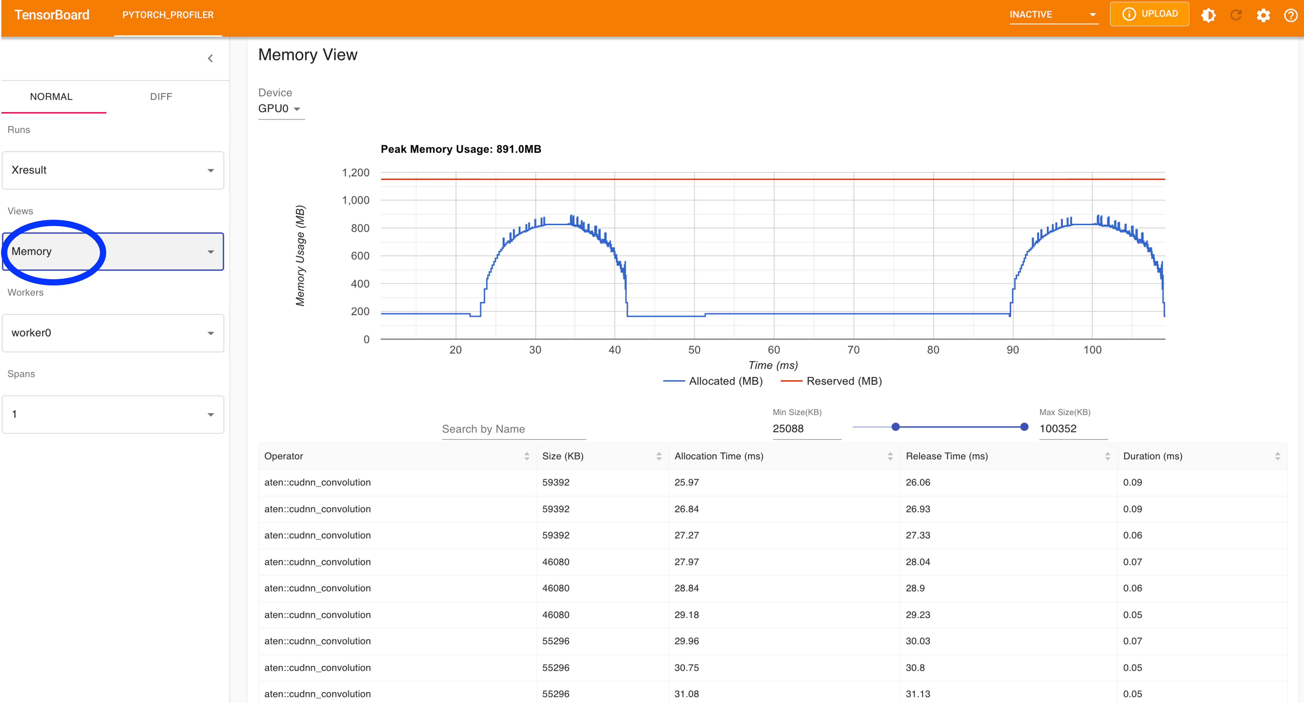
Fig 7: View of Memory usage.

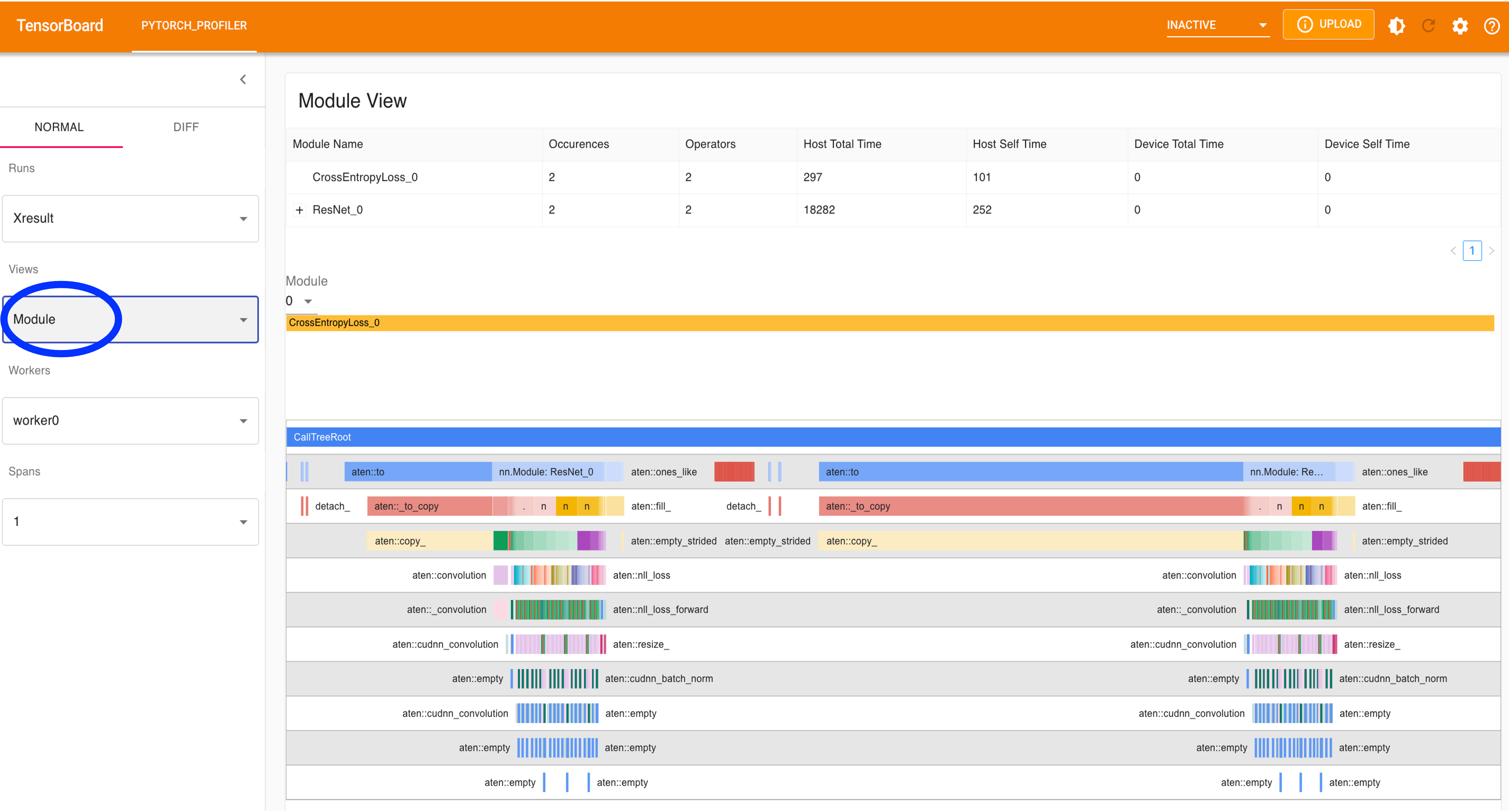
Fig 8: View of Modules.

Launching a PyTorch-based application

For completeness, we provide an example of a job script that incorporates a PyTorch singularity container. The script can be adapted according to requested computing resources.

#!/bin/bash -l
#SBATCH --job-name=PyTprofiler
#SBATCH --account=<project_account>
#SBATCH --time=00:10:00     #wall-time 
#SBATCH --partition=accel   #partition 
#SBATCH --nodes=1           #nbr of nodes
#SBATCH --ntasks=1          #nbr of tasks
#SBATCH --ntasks-per-node=1 #nbr of tasks per nodes (nbr of cpu-cores, MPI-processes)
#SBATCH --cpus-per-task=1   #nbr of threads
#SBATCH --gpus=1            #total nbr of gpus
#SBATCH --gpus-per-node=1   #nbr of gpus per node
#SBATCH --mem=4G            #main memory
#SBATCH -o PyTprofiler.out  #slurm output 

# Set up job environment
set -o errexit # exit on any error
set -o nounset # treat unset variables as error

#define paths
Mydir=<Path-to-Workspace>
MyContainer=${Mydir}/Container/pytorch_22.12-py3.sif
MyExp=${Mydir}/examples

#specify bind paths by setting the environment variable
#export SINGULARITY_BIND="${MyExp},$PWD"

#TF32 is enabled by default in the NVIDIA NGC TensorFlow and PyTorch containers 
#To disable TF32 set the environment variable to 0
#export NVIDIA_TF32_OVERRIDE=0

#to run singularity container 
singularity exec --nv -B ${MyExp},$PWD ${MyContainer} python ${MyExp}/resnet18_with_profiler_api.py

echo 
echo "--Job ID:" $SLURM_JOB_ID
echo "--total nbr of gpus" $SLURM_GPUS
echo "--nbr of gpus_per_node" $SLURM_GPUS_PER_NODE

More details about how to write a job script can be found here.

Conclusion

In conclusion, we have provided a guide on how to perform code profiling of GPU-accelerated Deep Learning models using the PyTorch Profiler. The particularity of the profiler relies on its simplicity and ease of use without installing additional packages and with a few lines of code to be added. These lines of code constitute the setting of the profiler, which can be customized according to the desired performance metrics. The profiler provides an overview of metrics; this includes a summary of GPU usage and Tensor cores usage (if it is enabled), this is in addition to an advanced analysis based on the view of GPU kernel, memory usage in time, trace and modules. These features are key elements for identifying bottlenecks in an application. Identifying these bottlenecks has the benefit of optimizing the application to run efficiently and reliably on HPC systems.

Relevant links

PyTorch Profiler

NVIDIA NGC container

Local port forwarding

Slides

PyTorch Profiler video